Module 4.2
Hypothesis Testing 2
Overview
In this module we extend hypothesis testing to comparisons between two groups. We use a permutation test to simulate the null distribution of a treatment effect and decide whether an observed difference is statistically significant. Our running example is a classic audit study examining racial discrimination in hiring.
Hypotheses for Group Comparisons
When comparing two groups, the null hypothesis states that there is no relationship between the grouping variable and the outcome — any observed difference is due to chance. The alternative hypothesis claims a genuine relationship exists.
The key insight behind permutation testing is that under the null hypothesis, the group labels do not matter. If treatment truly has no effect, we could randomly reassign group membership and the outcomes would look just the same. We exploit this to simulate the null distribution by shuffling the group labels many times and recomputing the difference in means each time.
The Résumé Experiment
Bertrand and Mullainathan sent 4,870 résumés to employers in Chicago and Boston, randomly assigning names associated with different racial backgrounds to otherwise identical applications. Because race was randomly assigned, any systematic difference in callback rates can be attributed to the racial associations of the names.
Let’s calculate callback rates by race and the treatment effect:
# A tibble: 2 × 2
  race   calls
  <chr>  <dbl>
1 black 0.0645
2 white 0.0965
mean_white <- means$calls[2]
mean_black <- means$calls[1]
teffect <- mean_white - mean_black
teffect[1] 0.03203285White-sounding names received callbacks at a rate roughly 3 percentage points higher than Black-sounding names.
Examining Estimates with Confidence Intervals
Before running a formal test, it is useful to visualize the point estimates and their uncertainty. We compute bootstrap confidence intervals for each group separately, then combine them for plotting:
ci_black <- resume_dta |>
  filter(race == "black") |>
  specify(response = received_callback) |>
  generate(reps = 10000, type = "bootstrap") |>
  calculate(stat = "mean") |>
  get_ci(level = 0.95)

ci_white <- resume_dta |>
  filter(race == "white") |>
  specify(response = received_callback) |>
  generate(reps = 10000, type = "bootstrap") |>
  calculate(stat = "mean") |>
  get_ci(level = 0.95)

plot_dta <- tibble(
  race     = c("Black", "White"),
  mean_calls = c(mean_black, mean_white),
  lower_95 = c(ci_black$lower_ci, ci_white$lower_ci),
  upper_95 = c(ci_black$upper_ci, ci_white$upper_ci)
)

ggplot(plot_dta, aes(x = race, y = mean_calls, ymin = lower_95, ymax = upper_95)) +
  geom_col(fill = "steelblue4") +
  geom_errorbar(width = 0.05) +
  ylim(0, 0.15) +
  labs(
    title = "Callback rates by race with 95% confidence intervals",
    x = "Race of Applicant",
    y = "Callback Rate"
  ) +
  theme_minimal()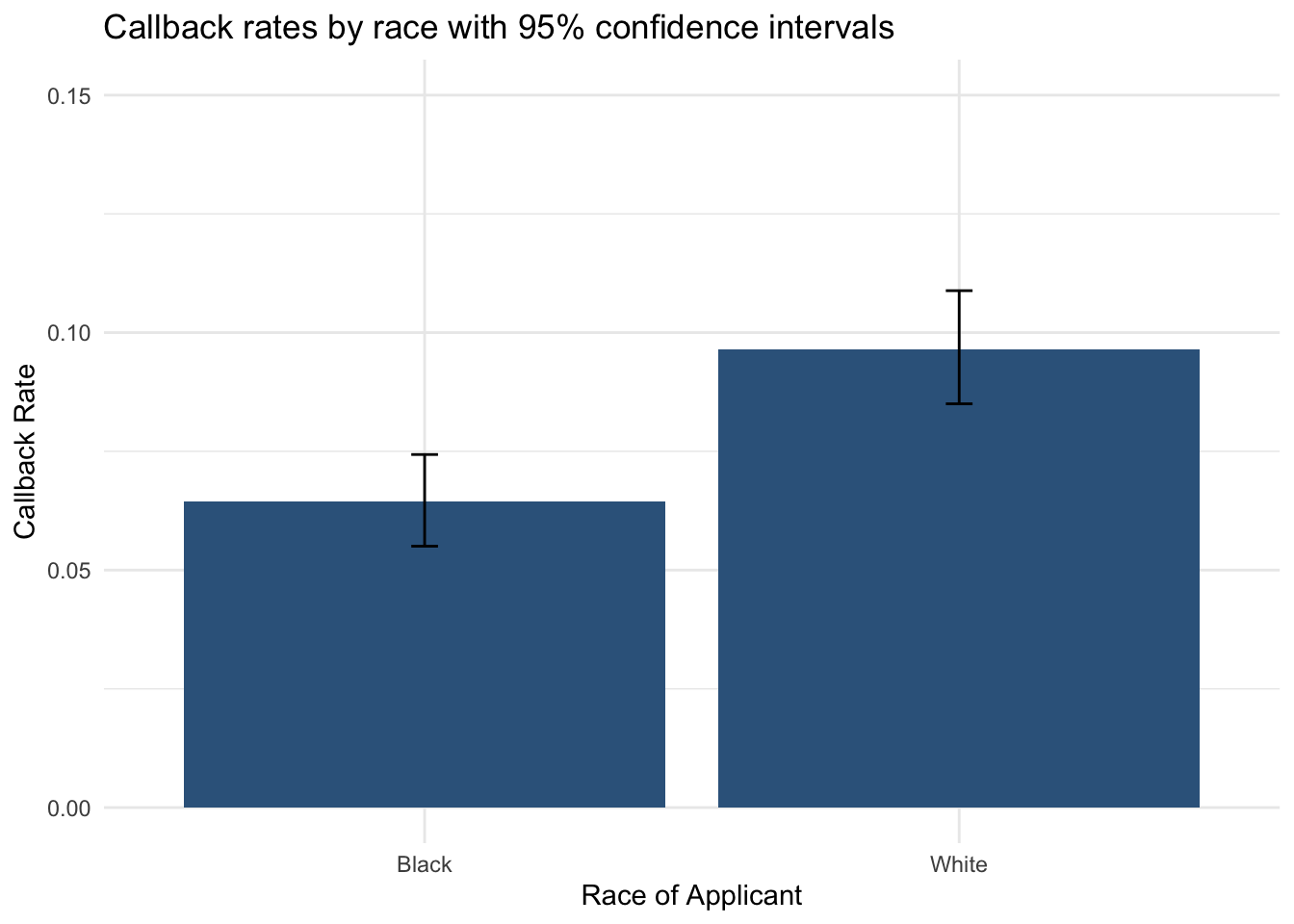
The non-overlapping confidence intervals already suggest a meaningful gap. But to formally test the null hypothesis we need a permutation test.
The Logic of Permutation Testing
We shuffle the race variable while keeping callback outcomes fixed, then recompute the difference in callback rates. This simulates what we would expect if race had no effect. Repeating thousands of times builds up the null distribution of treatment effects.
Here is the idea with a simplified six-applicant example:
Original data:
| Applicant | Race | Callback |
|---|---|---|
| A | Black | Yes |
| B | Black | No |
| C | Black | No |
| D | White | Yes |
| E | White | No |
| F | White | No |
After one shuffle:
| Applicant | Race (Shuffled) | Callback |
|---|---|---|
| A | White | Yes |
| B | Black | No |
| C | White | No |
| D | White | Yes |
| E | Black | No |
| F | Black | No |
We recalculate the difference in callback rates after each shuffle. If our real observed difference is extreme compared to this null distribution, we reject \(H_0\).
Implementing the Permutation Test
null_dist <- resume_dta |>
  specify(response = received_callback, explanatory = race) |>
  hypothesize(null = "independence") |>
  generate(reps = 10000, type = "permute") |>
  calculate(stat = "diff in means", order = c("white", "black"))

get_p_value(null_dist, obs_stat = teffect, direction = "greater")
# A tibble: 1 × 1
p_value
<dbl>
1 0You may see a message warning against reporting a p-value of exactly zero. This is an artifact of the number of permutations — with 10,000 reps, none happened to exceed the observed difference. Increasing reps to 100,000 would yield a very small but non-zero p-value.
visualize(null_dist) +
  shade_p_value(obs_stat = teffect, direction = "greater") +
  labs(
    title = "Null distribution with observed treatment effect",
    x = "Estimated Difference under the Null",
    y = "Count"
  ) +
  theme_minimal()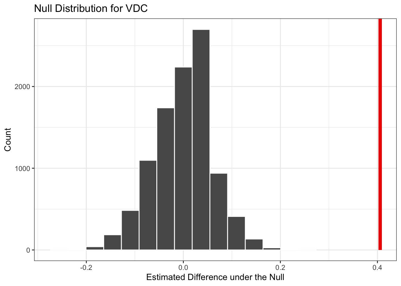
Drawing Conclusions
The p-value is effectively zero — none of the 10,000 permutations produced a racial gap as large as the one we observed. This is far below \(\alpha = 0.05\), so we reject the null hypothesis. The gap in callback rates between white- and Black-sounding names is extremely unlikely to have occurred by chance.
Because race was randomly assigned to the résumés, we can go a step further: this is not just a statistically significant association — it is evidence of causal racial discrimination in hiring. Random assignment is what makes this causal claim possible.