Before beginning this module, make sure you have reviewed:
The meaning of a proportion and sampling variability (Module 3.2)
The concepts of null and alternative hypotheses
What p-values and significance levels represent
Overview
In this module we introduce the concept of hypothesis testing — a framework for making inferences about a population parameter based on a sample statistic. We discuss the null and alternative hypotheses, the p-value, and the significance threshold. We then work through a concrete example involving a jobs training program to build intuition for how hypothesis testing works in practice.
Understanding Hypothesis Testing
Hypothesis testing is a method for deciding whether sample data provide convincing evidence against a default assumption about a population. That default assumption is the null hypothesis (\(H_0\)) — the “status quo” position that says nothing unusual is happening. The alternative hypothesis (\(H_A\)) is what we are actually trying to find evidence for: the claim that something is different.
The logic follows a proof-by-contradiction approach. We begin by assuming the null hypothesis is true, then ask: how likely would it be to observe data like ours if the null were really true? If our observed result would be perfectly ordinary under the null, we have no reason to doubt it — we fail to reject\(H_0\). But if our data would be extremely unlikely under the null, we take that as evidence against it — we reject\(H_0\) in favor of \(H_A\).
This probability — the chance of observing a result as extreme as ours, given that \(H_0\) is true — is the p-value. We compare it to a pre-specified significance level\(\alpha\) (most commonly 0.05). If \(p < \alpha\), we reject the null. If \(p \geq \alpha\), we fail to reject it.
Note that while \(\alpha = 0.05\) is conventional, it is also somewhat arbitrary. A result with \(p = 0.049\) and one with \(p = 0.051\) are substantively indistinguishable, even though they fall on opposite sides of the cutoff.
Your Turn
Think of a real-world claim you might want to test with hypothesis testing — a policy change, an intervention, a product claim, anything.
What is the null hypothesis? (What would “nothing going on” look like?)
What is the alternative hypothesis? (What are you trying to find evidence for?)
Is your alternative one-sided (the effect goes in a specific direction) or two-sided (any difference)?
A Jobs Training Program Example
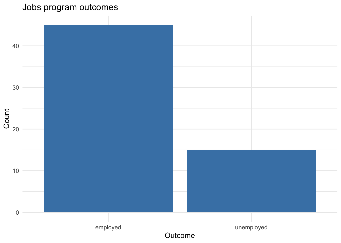
International development organizations sometimes run training programs to help people find employment. Suppose the national unemployment rate in a low-income country is 30%. One organization claims success because only 15 of the 60 people they trained ended up unemployed — a rate of 25%.
Is this a meaningful improvement? Or could this difference just be due to random chance? Let’s find out.
Null hypothesis (\(H_0: p = 0.30\)): The unemployment rate among program participants is no different from the national rate of 30%.
Alternative hypothesis (\(H_A: p < 0.30\)): The unemployment rate among participants is lower than the national rate.
Simulating the Null Distribution
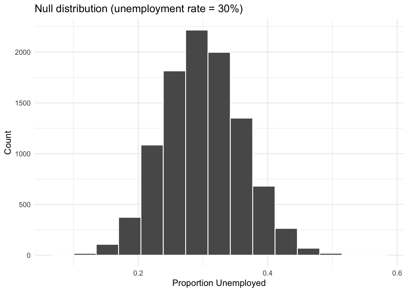
To test these hypotheses, we need to know what results we would expect to see if the null hypothesis were true. We simulate this by drawing many random samples under the assumption that the true unemployment rate is 30%. The distribution of those simulated proportions is the null distribution.
library(tidymodels)set.seed(42)null_dist<-jobs_program|>specify(response =outcome, success ="unemployed")|>hypothesize(null ="point", p =c("unemployed"=0.30, "employed"=0.70))|>generate(reps =10000, type ="draw")|>calculate(stat ="prop")null_dist|>summarize(mean =mean(stat))
# A tibble: 1 × 1
   mean
  <dbl>
1 0.300
null_dist|>visualize()+labs( title ="Null distribution (unemployment rate = 30%)", x ="Proportion Unemployed", y ="Count")+theme_minimal()
Calculating and Visualizing the P-value
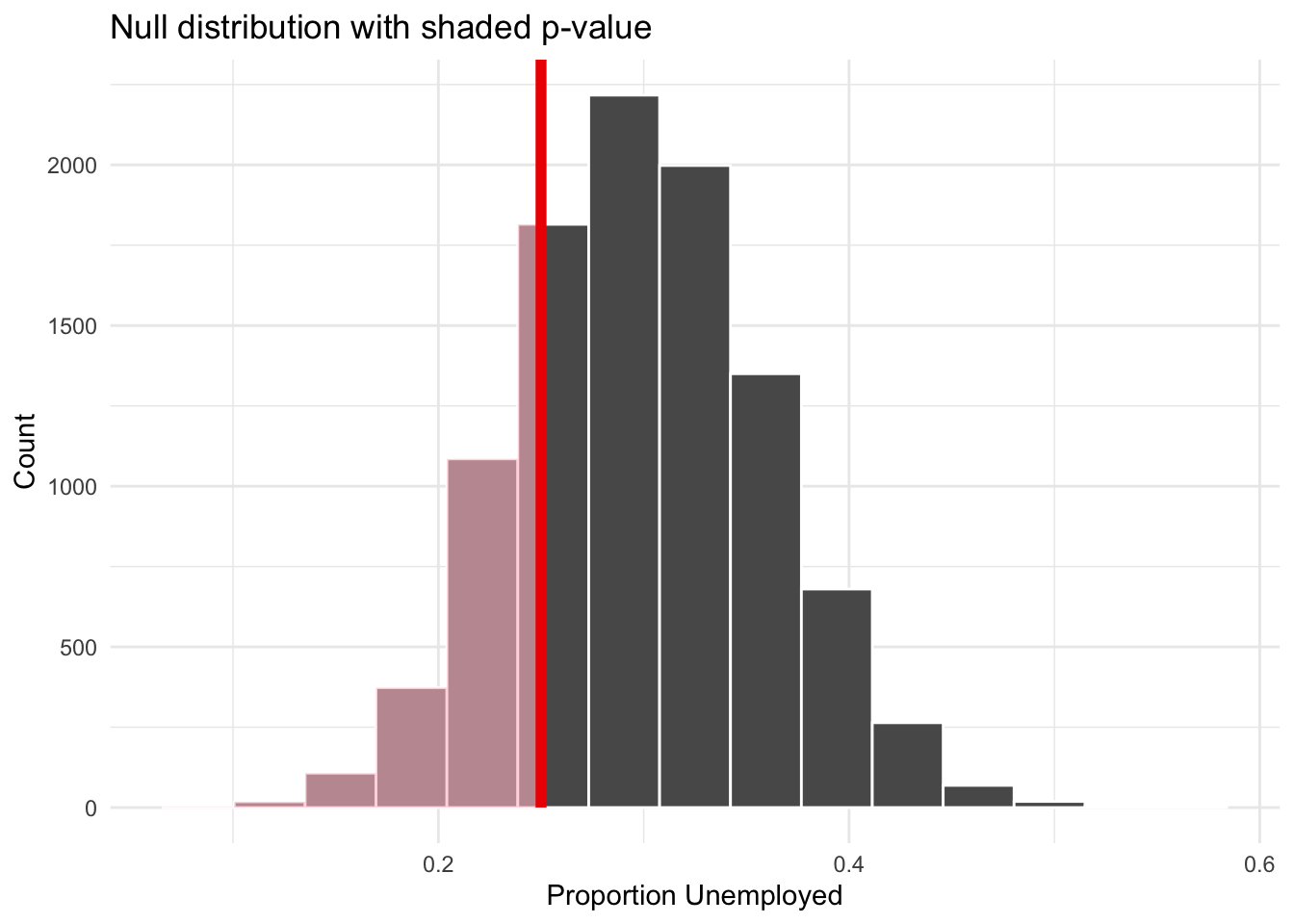
Our observed statistic is 15/60 = 0.25. The p-value tells us how often the null distribution produces a result this low or lower:
null_dist|>get_p_value(obs_stat =15/60, direction ="less")
# A tibble: 1 × 1
  p_value
    <dbl>
1   0.242
null_dist|>visualize()+shade_p_value(obs_stat =15/60, direction ="less")+labs( title ="Null distribution with shaded p-value", x ="Proportion Unemployed", y ="Count")+theme_minimal()
The p-value is around 0.23, meaning that if the true unemployment rate were 30% and we drew samples of 60 people, we would observe an unemployment rate as low as 25% about 23% of the time — purely by chance. Since 0.23 is well above \(\alpha = 0.05\), we fail to reject the null hypothesis. The program’s result is not statistically significant.
Note
Even if the p-value were below 0.05, we could not conclude that the program caused the reduction in unemployment. For a causal claim, we would need to know whether participants were randomly assigned to the program. Without randomization, there may be other factors — like motivation or prior skills — that explain who joined and who succeeded. Statistical significance tells us an effect is unlikely to be due to chance; it does not tell us why the effect exists.
Your Turn
What if the observed unemployment rate among participants were 10% instead of 25%? Re-run the test. Would you reject the null hypothesis?
Now try a different scenario: suppose the national rate is 50% and the observed rate in the program is 43%. Simulate the null distribution and decide: do you reject the null?