Think about sampling. What does the word “sample” mean to you? What is a sample you have encountered in your own life — and what larger group was it meant to represent?
Overview
In this module we explore statistical inference — the process of using a sample to make informed guesses about a broader population. Since we rarely have access to data on every individual in a population, we rely on samples to estimate quantities of interest, like proportions or averages.
But sampling introduces uncertainty. What if your sample is not typical? How much might your estimate differ if you sampled again? We will build intuition for what it means to sample from a population, how repeated sampling leads to a sampling distribution, and how to quantify uncertainty using standard errors and confidence intervals. We then explore two ways to construct CIs: using mathematical formulas, and using a computational approach called bootstrapping.
What Is Sampling?
Imagine trying to learn how many hours college students sleep each night. You could ask every student on Earth — but that is not practical. Instead you look at a smaller group that hopefully represents the whole: you take a sample.
The population is the full group you want to study. The sample is the smaller subset you actually observe. A parameter is a true (but usually unknown) characteristic of the population, like the actual average sleep time. A statistic is the number you compute from your sample — your estimate of that parameter. Inference is the process of using statistics to make educated guesses about parameters.
Target Population and Sampling Frame
In practice, it matters how the sample was drawn. The target population is the group you want to learn about. The sampling frame is the actual list or method used to select your sample. These often diverge:
Target population: All high school students in the U.S.
Sampling frame: Students in one school district’s enrollment database
When the sampling frame does not match the target population, we risk sampling bias — our estimates may not generalize to the group we actually care about. Keeping this distinction in mind is one of the most important habits of a careful data analyst.
Sampling Variability and Sampling Distributions
If you take one sample and compute a statistic, you get one answer. Take a different sample and you get a slightly different answer. This variability is unavoidable and forms the foundation of statistical inference.
If you repeated the sampling process many times, all those statistics would themselves form a distribution — the sampling distribution. Understanding the shape and spread of that distribution is what allows us to say how confident we are in any single estimate.
Activity: Sampling with M&Ms
Imagine a big bowl of M&Ms in front of you. Reach in and grab 20 at random, count how many are blue, and calculate the proportion. Put them back and grab 20 more. Repeat several times.
Each handful is a sample. Because you return the M&Ms each time, this is sampling with replacement. Notice how the proportion of blue M&Ms shifts from sample to sample — that variability is your sampling distribution in action.
If you have fun-size M&M packs at home, try this for real: record the proportion of blue M&Ms in each pack in a CSV file, load it in R, and make a histogram. Then take the average across all your proportions. How close does it come to the known population proportion of blue M&Ms (about 24%)?
This simple activity captures exactly what we mean by repeated sampling and bootstrap distributions.
Standard Error
The spread of the sampling distribution has a special name: the standard error (SE). It tells us, on average, how much a statistic varies from one sample to another. A smaller SE means more precise estimates; a larger SE means more variability.
Standard error depends on two things: sample size and variability in the data. Bigger samples produce smaller standard errors — as you collect more data, your estimate converges toward the true parameter and the sampling distribution narrows.
Understanding standard error is the key to constructing confidence intervals, which we turn to next.
Confidence Intervals
A confidence interval gives us a range of values within which we believe the true population parameter likely falls. It is built from the sample statistic and its standard error.
When we report a 95% confidence interval we say we are “95% confident” that the true parameter lies within the interval. More precisely: if we repeated our sampling many times and computed a CI each time, about 95% of those intervals would contain the true parameter. It is not a statement that the parameter has a 95% probability of being in this particular interval — the parameter is fixed; our interval is what varies.
There are two ways to construct confidence intervals: using mathematical formulas, or using a computational approach called bootstrapping.
Math-Based Confidence Intervals
The normal approximation method uses the Central Limit Theorem, which tells us that for large enough samples the sampling distribution of the mean is approximately normal. The general formula is:
\[\text{CI} = \hat{x} \pm z \times \text{SE}\]
where \(\hat{x}\) is the sample statistic, SE is the standard error, and \(z\) depends on the confidence level:
95% confidence → \(z \approx 1.96\)
90% confidence → \(z \approx 1.645\)
For a proportion, the standard error is:
\[SE = \sqrt{\frac{\hat{p}(1 - \hat{p})}{n}}\]
Worked example. Suppose we survey 100 people and 64 say they like pineapple on pizza. Our sample proportion is \(\hat{p} = 0.64\).
We are 95% confident that between 54.6% and 73.4% of the population likes pineapple on pizza.
Two intuitions to take away: the larger the standard error, the wider the CI. And the larger the sample size \(n\), the smaller the SE — and therefore the narrower and more precise the CI.
Bootstrapping
Bootstrapping is a computational alternative to math-based CIs. It repeatedly resamples with replacement from the observed data to approximate the sampling distribution — no normality assumption required.
The logic: your original sample is the best approximation of the population you have. By randomly resampling from it, you simulate what other samples might look like. Computing the statistic on each resample builds up a bootstrap distribution, from which you read off the CI directly.
Reasons to prefer bootstrapping:
It does not require assumptions about the shape of the population distribution.
It works well even with small samples or skewed data.
It is straightforward to implement in R using the infer package.
Worked Example: Russian Survey Data
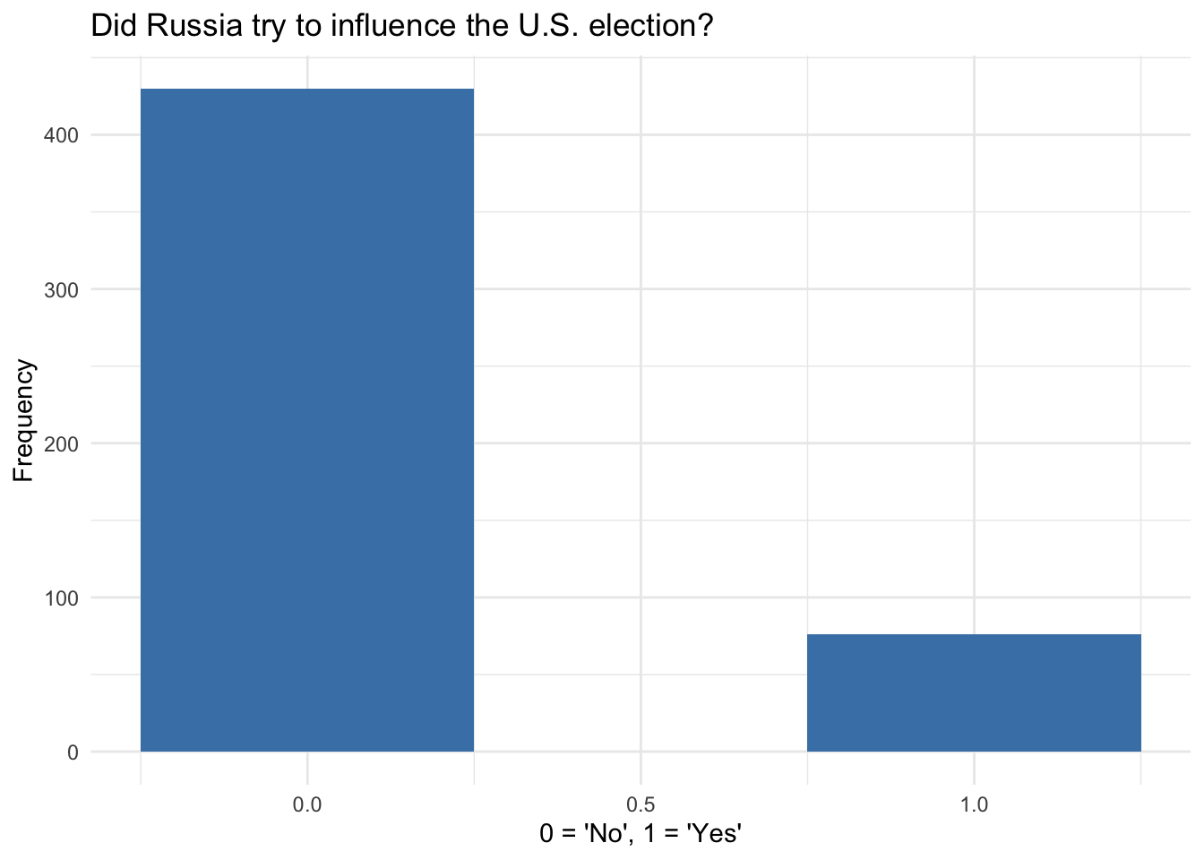
The openintro package contains a Pew Research survey of 506 Russians asked whether they believed their country tried to interfere in the 2016 U.S. presidential election. We recode the response as a binary variable and summarize:
# A tibble: 1 × 2
   mean    sd
  <dbl> <dbl>
1 0.150 0.358
ggplot(russiaData, aes(x =try_influence))+geom_bar(fill ="steelblue", width =0.5)+labs( title ="Did Russia try to influence the U.S. election?", x ="0 = 'No', 1 = 'Yes'", y ="Frequency")+theme_minimal()
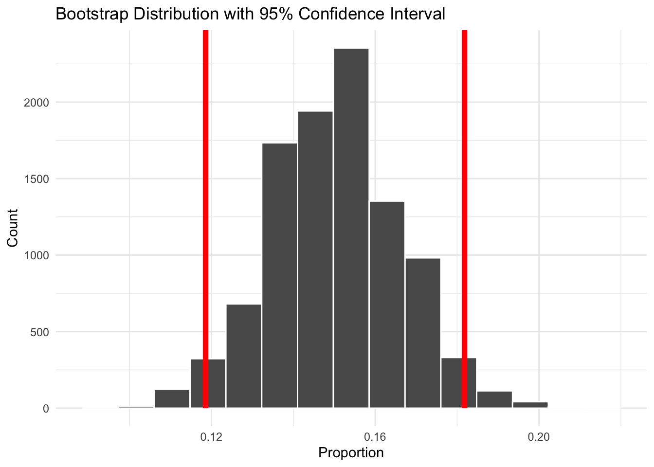
Now we build the bootstrap distribution using tidymodels. The pipeline is: specify() the variable of interest → generate() many bootstrap resamples → calculate() the statistic on each one:
library(tidymodels)set.seed(66)boot_dist<-russiaData|>specify(response =try_influence)|>generate(reps =10000, type ="bootstrap")|>calculate(stat ="mean")glimpse(boot_dist)
boot_dist|>visualize()+shade_ci(ci, color ="red", fill =NULL)+labs( title ="Bootstrap Distribution with 95% Confidence Interval", x ="Proportion", y ="Count")+theme_minimal()
Note
visualize() returns a ggplot2 object, so you can add layers to it — labels, themes, annotations — using the standard ggplot2 syntax.
The shaded region marks the 95% confidence interval for the proportion of Russians who believe their country interfered in the election.
Your Turn
The 95% CI is printed in the ci object above. Which of the following is the correct interpretation?
95% of the time, the percentage of Russians who believe Russia interfered is between these values.
95% of all Russians believe the probability of interference is within the interval.
We are 95% confident that the proportion of Russians who believe Russia interfered in the 2016 election is between these values.
We are 95% confident that the proportion of Russians who supported interference is between these values.
Code
# The correct answer is (c). The CI gives a range of plausible values for the# population proportion based on this sample. It does not describe individual# beliefs (b, d), nor does it mean the parameter literally varies (a).