Module 11.1
Logistic Regression: Motivation and Model
Prework
- Install the
peacesciencerpackage (install.packages("peacesciencer")) - Have a look at the
peacesciencerdocumentation to familiarize yourself with its contents and basic functions
Overview
So far in our data science journey, we’ve focused on modeling continuous numerical outcomes like income, temperature, or test scores. But many of the most interesting questions in research involve outcomes that are binary: yes or no, success or failure, presence or absence.
In this module, we will explore why we need a different modeling approach when our outcome variable is binary rather than continuous. We will use the compelling example of civil war onset to understand the conceptual foundations that motivate logistic regression, setting the stage for the technical details that we will cover in upcoming modules. By the end of this module, you’ll be able to distinguish between continuous and binary outcome variables, understand why linear regression is inappropriate for binary outcomes, grasp the concept of Bernoulli trials in the context of real research, appreciate why probabilities must be constrained between 0 and 1, and recognize when a different modeling approach is needed.
From Continuous to Binary Outcomes
Throughout our exploration of linear regression, we’ve been working with continuous numerical outcomes. These are variables that can theoretically take on any value within a range, like someone’s height (5.8 feet, 5.83 feet, 5.834 feet), annual income ($45,000, $45,231, $45,231.67), or a test score that could be anywhere from 0 to 100.
But many research questions center on outcomes that are fundamentally different: binary outcomes. These variables have exactly two possible values, often coded as yes/no, success/failure, present/absent, or simply 1/0. Consider research questions like whether a patient recovers from treatment, whether a voter turns out for an election, whether an email gets classified as spam, or whether a student graduates within four years. Each of these involves a binary outcome where there are only two possibilities for each observation.
Let’s examine an example from political science research that perfectly illustrates why we need different modeling approaches for binary outcomes. The research question is straightforward: did a civil war begin in a given country in a given year?
This question was central to groundbreaking research by Fearon and Laitin (2003), who wanted to understand what factors make civil war more or less likely to begin. For any country in any year, there are only two possibilities: either a civil war began (coded as 1, or “success” in statistical terms) or no civil war began (coded as 0, or “failure”). Note that calling conflict onset a “success” might feel strange since we’re certainly not celebrating war! In statistics, “success” simply refers to the outcome we’re modeling, regardless of whether it’s socially desirable.
Researchers hypothesized that various factors might influence the probability of conflict onset, including economic wealth (GDP per capita), level of democracy, mountainous terrain (which might facilitate insurgency), ethnic diversity, population size, and previous conflict history. The key insight is that we want to model how these factors influence the probability that conflict will begin, not predict an exact numerical outcome.
The Problem with Linear Regression for Binary Data
Now comes the crucial question: why can’t we just use regular linear regression for binary outcomes?
Think about what linear regression does. It creates a straight line that predicts numerical values based on our predictors. For our conflict example, a linear model might look like:
\[\text{Conflict Onset} = \beta_0 + \beta_1(\text{GDP per capita}) + \beta_2(\text{Democracy level}) + \beta_3(\text{Terrain roughness}) + \ldots\]
But there is a fundamental problem here. Linear regression can predict any value along a continuous range. It might predict that a country has a “-0.3” probability of conflict onset, or a “1.7” probability.
What does it mean for something to have a 170% chance of happening? Or a negative probability? These predictions are mathematically nonsensical because probabilities must be constrained between 0 and 1 (or 0% and 100%).
Another problem with applying linear regression to a binary outcome is that it can shift the decision boundary in unstable ways. Linear regression implicitly uses the point where the predicted value crosses 0.5 as the cutoff for classifying an observation as “success” or “failure.”
Let’s assume one predictor has an extreme value — for example, Nepal’s very mountainous terrain — this can pull the fitted line up or down, shifting the decision boundary along the predictor axis. As a result, cases that should be classified as high risk for conflict might now be on the wrong side of the boundary and be misclassified as low risk. Logistic regression addresses this problem by directly modeling the probability and keeping the decision boundary consistent and interpretable.
Bernoulli Trials and Probability Modeling
To properly model binary outcomes, we should think about each observation as a Bernoulli trial. A Bernoulli trial is a random experiment with exactly two possible outcomes (success and failure), where the probability of success remains constant for that specific trial. A classic example is a fair coin flip: heads (success) or tails (failure), with a fixed 50% chance of success.
In our conflict onset example, each country-year combination represents a separate Bernoulli trial:
- Afghanistan in 2001: One trial with its own probability of conflict onset
- Switzerland in 2001: A different trial with its own (likely much lower) probability
- Afghanistan in 2002: Yet another trial with its own probability
The key insight is that while each trial has only two possible outcomes, the probability of “success” can vary between trials based on the specific circumstances (the predictor variables) of that country in that year.
Mathematically, we can express this as:
\[y_i \sim \text{Bernoulli}(p_i)\]
This notation means that each outcome \(y_i\) follows a Bernoulli distribution with its own probability \(p_i\).
Generalized Linear Models
Our exploration reveals that we need a modeling framework that can handle binary outcome variables appropriately, ensure predicted probabilities stay between 0 and 1, allow different observations to have different success probabilities, and incorporate multiple predictor variables in a systematic way.
This is where Generalized Linear Models (GLMs) come in. GLMs provide a suitable framework for extending regression concepts beyond continuous outcomes. Rather than forcing binary data into an inappropriate linear framework, GLMs use mathematical transformations that naturally respect the constraints of probability.
All GLMs share three key characteristics:
A probability distribution that describes how the outcome variable is generated (for binary outcomes, this is the Bernoulli distribution)
-
A linear model that combines predictor variables:
\[\eta = \beta_0 + \beta_1 X_1 + \beta_2 X_2 + \ldots + \beta_k X_k\]
A link function that connects the linear model to the parameter of the outcome distribution (ensuring probabilities stay between 0 and 1)
A link function is a mathematical function that connects the linear model (which can range from −∞−∞ to +∞+∞) to the parameter of the outcome distribution (such as the probability of success) in a way that respects its natural constraints. For binary outcomes, the link function ensures that the linear combination of predictors maps to a probability between 0 and 1.
Logistic regression is one of the most common and useful examples of a GLM. It uses a special mathematical transformation (the logistic function) that takes any real number from the linear model and converts it to a probability between 0 and 1.
Summary and Looking Ahead
In this module, we have explored why binary outcomes require a different modeling approach than continuous variables. We saw that many important research questions involve binary rather than continuous outcomes, and that linear regression fails for binary data because it can produce impossible probability predictions. We learned to think of each observation as a Bernoulli trial with its own success probability and to recognize that we need a modeling framework that respects probability constraints while incorporating multiple predictors.
Logistic regression, as part of the GLM family, provides exactly this framework. It allows us to model how various factors influence the probability of binary outcomes while ensuring our predictions remain mathematically sensible. In our next modules, we will dive into the mathematical details of how logistic regression works, learn to fit and interpret these models, and practice making predictions with real data.
The Logistic Regression Model
The Sigmoid Function: The Key to Valid Probabilities
Remember our fundamental problem from Module 5.1: linear regression can predict impossible probabilities like -0.3 or 1.7 when we apply it to binary outcomes. We need a mathematical function that can take any real number (from negative infinity to positive infinity) and transform it into a valid probability between 0 and 1.
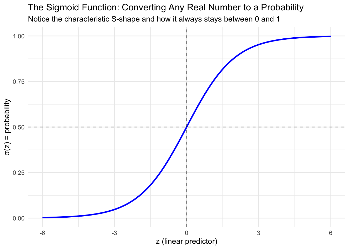
Enter the sigmoid function (also called the logistic function). The sigmoid function is defined as:
\[\sigma(z) = \frac{1}{1 + e^{-z}}\]
where \(z\) can be any real number, and \(\sigma(z)\) will always be between 0 and 1.
Let’s visualize what this function looks like:
The sigmoid function has several important properties that make it perfect for our needs. Most importantly, it always produces outputs between 0 and 1, no matter what value we put in for \(z\). The function has a characteristic S-shaped curve that rises slowly at first, then more rapidly in the middle, then slowly again as it approaches its limits. It’s symmetric around 0.5, meaning that when \(z = 0\), we get \(\sigma(z) = 0.5\). Unlike a step function that would create abrupt jumps, the sigmoid provides smooth probability transitions as our predictors change.
This is exactly what we need for binary classification! The sigmoid function takes our linear combination of predictors (which can be any value) and converts it to a probability.
The Logit Function: The Other Side of the Equation
While the sigmoid function shows us how to convert linear predictors to probabilities, we actually need to set up our model the other way around. Remember that in regression, we want to model something as a linear function of our predictors. But we can’t model probabilities directly as linear functions because probabilities are constrained between 0 and 1, while linear functions can produce any value from negative infinity to positive infinity.
This is where we need to “go the other direction” - we need a function that takes probabilities and transforms them onto an unrestricted scale where we can model them linearly. The logit function does exactly this transformation:
\[\text{logit}(p) = \log\left(\frac{p}{1-p}\right)\]
The logit function takes a probability (between 0 and 1) and transforms it to any real number (between negative and positive infinity). Let’s visualize this:
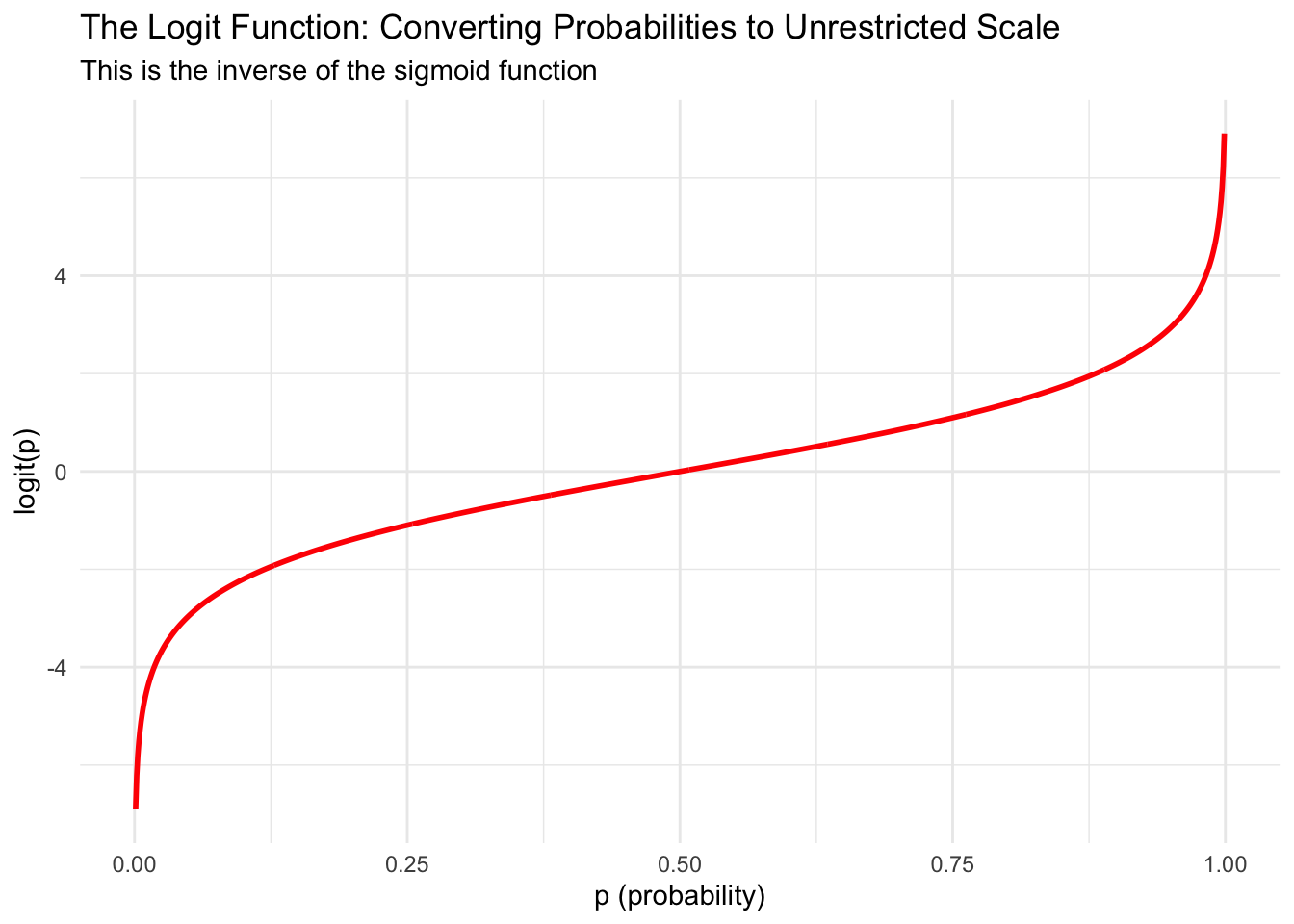
The term \(\frac{p}{1-p}\) in the logit function is called the odds. When \(p = 0.5\) (equal chance of success and failure), the odds equal 1, and \(\log(1) = 0\). When \(p > 0.5\), the odds are greater than 1, and the logit is positive. When \(p < 0.5\), the odds are less than 1, and the logit is negative.
The Complete Logistic Regression Model
Now we can put together the complete picture of how logistic regression works. Remember from Module 5.1 that all GLMs have three components:
- Distribution: \(y_i \sim \text{Bernoulli}(p_i)\) (each observation is a Bernoulli trial)
- Linear predictor: \(\eta_i = \beta_0+ \beta_1 x_{1,i} + \cdots + \beta_k x_{k,i}\) (familiar linear combination)
- Link function: \(\text{logit}(p_i) = \eta_i\) (connects the linear predictor to the probability)
Putting it all together:
\[\text{logit}(p_i) = \eta_i = \beta_0+ \beta_1 x_{1,i} + \cdots + \beta_k x_{k,i}\]
To get back to probabilities, we apply the sigmoid function:
\[p_i = \sigma(\eta_i) = \frac{1}{1 + e^{-(\beta_0+ \beta_1 x_{1,i} + \cdots + \beta_k x_{k,i})}}\]
Or an equivalent form that is often used in practice:
\[p_i = \frac{\exp(\beta_0+\beta_1 x_{1,i} + \cdots + \beta_k x_{k,i})}{1+\exp(\beta_0+\beta_1 x_{1,i} + \cdots + \beta_k x_{k,i})}\]
The key insight is that we model the logit of the probability as a linear function of our predictors, then use the sigmoid function to convert back to probabilities that make sense. The logit gets us from constrained probabilities to an unrestricted scale where we can do linear modeling, and the sigmoid gets us back from that unrestricted scale to meaningful probabilities.
Worked Example: Logistic Regression with Conflict Onset Data
Let’s implement logistic regression using our conflict onset example. We can use data from the peacesciencer package. The create_stateyears() function will help us set up a dataset where each row represents one country in one year, and our binary outcome variable will indicate whether a civil war began in that country in that year. Then we add different sets of predictors using peacesciencer “add” functions like add_ucdp_acd(), add_democracy(), and others to create a rich dataset for our analysis.
library(peacesciencer)
library(dplyr)

# Create the conflict dataset
conflict_df <- create_stateyears(system = 'gw') |>
  filter(year %in% c(1946:1999)) |>
  add_ucdp_acd(type=c("intrastate"), only_wars = FALSE) |>
  add_democracy() |>
  add_creg_fractionalization() |>
  add_sdp_gdp() |>
  add_rugged_terrain()

# Take a look at our data
glimpse(conflict_df)
Rows: 7,624
Columns: 22
$ gwcode <dbl> 2, 2, 2, 2, 2, 2, 2, 2, 2, 2, 2, 2, 2, 2, 2, 2, 2, 2, 2…
$ gw_name <chr> "United States of America", "United States of America",…
$ microstate <dbl> 0, 0, 0, 0, 0, 0, 0, 0, 0, 0, 0, 0, 0, 0, 0, 0, 0, 0, 0…
$ year <dbl> 1946, 1947, 1948, 1949, 1950, 1951, 1952, 1953, 1954, 1…
$ ucdpongoing <dbl> 0, 0, 0, 0, 0, 0, 0, 0, 0, 0, 0, 0, 0, 0, 0, 0, 0, 0, 0…
$ ucdponset <dbl> 0, 0, 0, 0, 0, 0, 0, 0, 0, 0, 0, 0, 0, 0, 0, 0, 0, 0, 0…
$ maxintensity <dbl> NA, NA, NA, NA, NA, NA, NA, NA, NA, NA, NA, NA, NA, NA,…
$ conflict_ids <chr> NA, NA, NA, NA, NA, NA, NA, NA, NA, NA, NA, NA, NA, NA,…
$ euds <dbl> 1.293985, 1.308359, 1.343539, 1.330836, 1.354015, 1.350…
$ aeuds <dbl> 0.4862558, 0.5006298, 0.5358093, 0.5231064, 0.5462858, …
$ polity2 <dbl> 9, 9, 9, 9, 9, 9, 9, 9, 9, 9, 9, 9, 9, 9, 9, 9, 9, 9, 9…
$ v2x_polyarchy <dbl> 0.603, 0.607, 0.599, 0.580, 0.585, 0.611, 0.611, 0.612,…
$ ethfrac <dbl> 0.2226323, 0.2248701, 0.2271561, 0.2294918, 0.2318781, …
$ ethpol <dbl> 0.4152487, 0.4186156, 0.4220368, 0.4255134, 0.4290458, …
$ relfrac <dbl> 0.4980802, 0.5009111, 0.5037278, 0.5065309, 0.5093204, …
$ relpol <dbl> 0.7769888, 0.7770017, 0.7770303, 0.7770729, 0.7771274, …
$ wbgdp2011est <dbl> 28.539, 28.519, 28.545, 28.534, 28.572, 28.635, 28.669,…
$ wbpopest <dbl> 18.744, 18.756, 18.781, 18.804, 18.821, 18.832, 18.848,…
$ sdpest <dbl> 28.478, 28.456, 28.483, 28.469, 28.510, 28.576, 28.611,…
$ wbgdppc2011est <dbl> 9.794, 9.762, 9.764, 9.730, 9.752, 9.803, 9.821, 9.857,…
$ rugged <dbl> 1.073, 1.073, 1.073, 1.073, 1.073, 1.073, 1.073, 1.073,…
$ newlmtnest <dbl> 3.214868, 3.214868, 3.214868, 3.214868, 3.214868, 3.214…# Check our binary outcome variable
table(conflict_df$ucdponset, useNA = "always")
   0    1 <NA>
7481  143    0
Understanding the Code
In the last line, we use the table() function to summarize our binary outcome variable ucdponset, which indicates whether a civil war began in that country in that year. The useNA = "always" argument ensures we also see how many observations have missing values. this helps us understand the distribution of our outcome variable, how many observations we have in total and whether we have any missing data that we need to be concerned with before running our regressions.
Take a moment to examine this output. Consider how many observations we have and what our binary outcome variable is called. Notice the distribution of 1s versus 0s in the outcome variable. Most importantly, think about what each row represents in terms of Bernoulli trials.
Remember, each row represents one country in one year, and we’re asking: “Did a civil war begin in this country in this year?” Each observation is a separate Bernoulli trial with its own probability of “success” (conflict onset) based on that country’s characteristics in that year.
Running a Logistic Regression in R
The good news is that implementing logistic regression in R is very similar to linear regression. We just need to make a few changes to tell R that we are working with a binary outcome. Instead of using
lm(continuous_outcome ~ predictor1 + predictor2, data = mydata)
as we did for linear regression, we now use
glm(binary_outcome ~ predictor1 + predictor2, data = mydata, family = "binomial")
for logistic regression.
The key changes are switching from lm() to glm() and adding the family = "binomial" argument to specify we’re working with binary data. This family specification tells R to use the logit link function automatically, handling all the mathematical transformations we discussed.
Let’s start with a simple bivariate example, examining how GDP per capita relates to conflict onset:
# Fit a logistic regression model
conflict_model <- glm(ucdponset ~ wbgdppc2011est,
                      data = conflict_df,
                      family = "binomial")

# Look at the summary
summary(conflict_model)
Call:
glm(formula = ucdponset ~ wbgdppc2011est, family = "binomial",
    data = conflict_df)

Coefficients:
               Estimate Std. Error z value Pr(>|z|)
(Intercept)    -1.00735    0.41297  -2.439   0.0147 *
wbgdppc2011est -0.35695    0.05089  -7.015 2.31e-12 ***
---
Signif. codes:  0 '***' 0.001 '**' 0.01 '*' 0.05 '.' 0.1 ' ' 1

(Dispersion parameter for binomial family taken to be 1)

    Null deviance: 1420.5  on 7623  degrees of freedom
Residual deviance: 1381.9  on 7622  degrees of freedom
AIC: 1385.9

Number of Fisher Scoring iterations: 7
The output looks similar to linear regression, but the interpretation is different because we’re modeling the log-odds (logit) rather than the outcome directly.
Understanding the Model Output
When you look at the summary output from a logistic regression, remember that the coefficients are on the log-odds scale. A coefficient of 0.5 means a one-unit increase in that predictor increases the log-odds by 0.5. The intercept represents the log-odds of the outcome when all predictors equal zero. Standard errors and p-values are interpreted similarly to linear regression for hypothesis testing, but you won’t see an R-squared value since we don’t use that measure of fit with logistic regression.
The coefficients tell us about direction and significance, but interpreting the magnitude on the log-odds scale can be challenging. This is why we typically transform these results into more intuitive measures when making practical interpretations.
Summary and Looking Ahead
In this module, we’ve explored the mathematical foundations that make logistic regression work. The sigmoid function provides the crucial capability to transform any real number into a valid probability between 0 and 1, while the logit function allows us to transform probabilities into an unrestricted scale that we can model linearly. Together, these functions enable the complete GLM framework that connects our linear predictors to binary outcomes through the logit link function. Implementing this approach in R requires only small changes from linear regression, using glm() with family = "binomial" instead of our familiar lm() function.
In our next module, we’ll learn how to interpret these log-odds coefficients in more meaningful ways through odds ratios and predicted probabilities. We will discover how to answer questions like “How much does democracy change the probability of conflict onset?” and “What’s the predicted probability of conflict for a specific country profile?” Thanfully, the mathematical foundation that we laid today will make those interpretations much clearer and more intuitive.
References
Fearon, James D., and David D. Laitin. 2003. “Ethnicity, Insurgency, and Civil War.” American Political Science Review 97 (1): 75–90. https://doi.org/10.1017/S0003055403000534.