Regression Tables

How to Interpret and Create

April 23, 2024

Multiple Logistic Regression

Multiple Logistic Regression

• Just as with linear models, we can also run multiple logistic regressions
• We can include multiple predictors in the model
• Usually we want to include our main predictor of interest and control variables
• The interpetation of the coefficients is the same as in the bivariate models

Download the data using the peacesciencer package if you haven’t already…

conflict_df <- create_stateyears(system = 'gw') |>
  filter(year %in% c(1946:1999)) |>
  add_ucdp_acd(type=c("intrastate"), only_wars = FALSE) |>
  add_democracy() |>
  add_creg_fractionalization() |>
  add_sdp_gdp() |>
  add_rugged_terrain()

Example, including multiple predictors associated with conflict:

conflict_model <- logistic_reg() |>
  set_engine("glm") |>
  fit(factor(ucdponset) ~ ethfrac + relfrac + v2x_polyarchy + 
                          rugged + wbgdppc2011est + wbpopest,
                  data= conflict_df,
                  family = "binomial")

tidy(conflict_model)

# A tibble: 7 × 5
  term           estimate std.error statistic   p.value
  <chr>             <dbl>     <dbl>     <dbl>     <dbl>
1 (Intercept)     -5.69      1.41      -4.04  0.0000527
2 ethfrac          0.800     0.381      2.10  0.0356   
3 relfrac         -0.391     0.417     -0.939 0.348    
4 v2x_polyarchy   -0.602     0.509     -1.18  0.237    
5 rugged           0.0641    0.0760     0.843 0.399    
6 wbgdppc2011est  -0.372     0.121     -3.08  0.00204  
7 wbpopest         0.293     0.0673     4.35  0.0000134

Predicted Probabilities

# load the 
library(marginaleffects)

# seledct some countries for a given year
selected_countries <- conflict_df |>
  filter(
    statename %in% c("United States of America", "Venezuela", "Rwanda"),
    year == 1999)

# extract the model
conflict_fit <- conflict_model$fit

# calculate margins for the subset
marg_effects <- predictions(conflict_fit, newdata = selected_countries)

# tidy the results
tidy(marg_effects) |>
  select(estimate, p.value, conf.low, conf.high, statename)

# A tibble: 3 × 5
  estimate  p.value conf.low conf.high statename               
     <dbl>    <dbl>    <dbl>     <dbl> <chr>                   
1   0.0123 2.23e-28  0.00567    0.0264 United States of America
2   0.0140 2.25e-70  0.00879    0.0222 Venezuela               
3   0.0286 8.46e-39  0.0170     0.0477 Rwanda                  

Your Turn!

• Run a multivariate logistic model using conflict onset as the outcome variable
• Select alternative variables and/or alternative measures of the same variables
• Interpret some of the coefficients
• Calculate the precicted probability in a handful of country-years based on your analysis

10:00

Regression Tables

What’s in a Regression Table?

Regression Tables with modelsummary

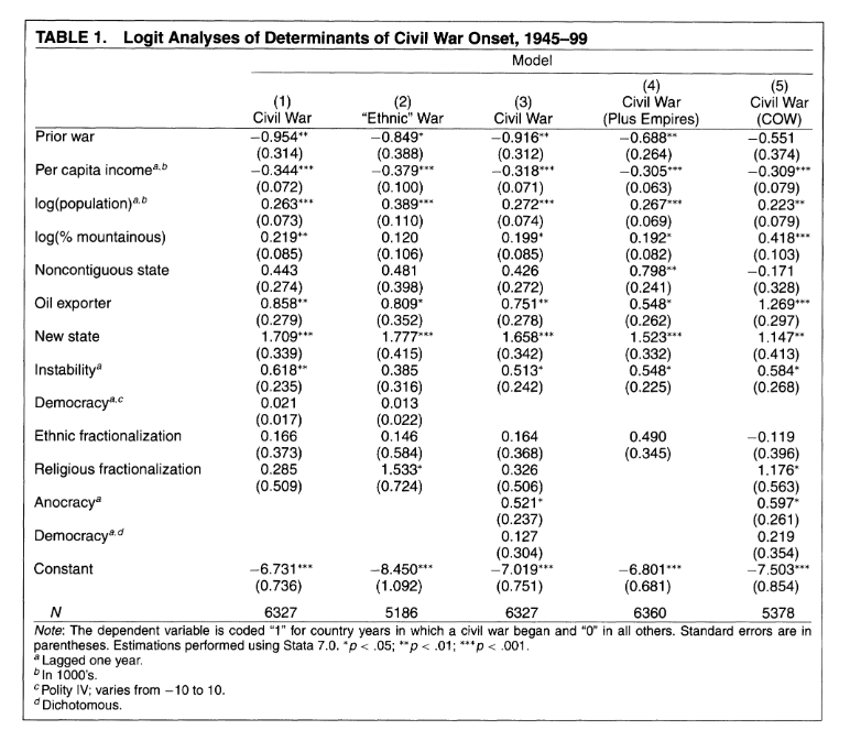
• Oftentimes we want to show multiple models at once (like F&L)
• We want to compare across them and see which is the best model
• How can we do that?
• There are many ways to do this in R
• We will use the modelsummary package

Run Multiple Models

ethnicity <- glm(ucdponset ~ ethfrac + relfrac + wbgdppc2011est + wbpopest, # store each model in an object
                  data = conflict_df,
                  family = "binomial")

democracy <- glm(ucdponset ~ v2x_polyarchy + wbgdppc2011est +  wbpopest,
                  data = conflict_df,
                  family = "binomial")

terrain <- glm(ucdponset ~ rugged + wbgdppc2011est + wbpopest ,
                  data = conflict_df,
                  family = "binomial")

full_model <- glm(ucdponset ~ ethfrac + relfrac + v2x_polyarchy + rugged +
                        wbgdppc2011est + wbpopest,
                  data = conflict_df,
                  family = "binomial")

Prep Data for Display

models <- list("Ethnicity" = ethnicity,  # store list of models in an object
               "Democracy" = democracy, 
               "Terrain" = terrain, 
               "Full Model" = full_model)

coef_map <- c("ethfrac" = "Ethnic Frac",  # map coefficients
        "relfrac" = "Religions Frac",     #(change names and order)
        "v2x_polyarchy" = "Polyarchy",
        "rugged" = "Terrain",
        "wbgdppc2011est" = "Per capita GDP",
        "wbpopest" = "Population",
        "(Intercept)" = "Intercept")

caption = "Table 1: Predictors of Conflict Onset" # store caption
reference = "See appendix for data sources."      # store reference notes

Display the Models

Table 1: Predictors of Conflict Onset

	Ethnicity	Democracy	Terrain	Full Model
+ p < 0.1, * p < 0.05, ** p < 0.01, *** p < 0.001
See appendix for data sources.
Ethnic Frac	0.744*			0.800*
	(0.367)			(0.381)
Religions Frac	-0.481			-0.391
	(0.411)			(0.417)
Polyarchy		-0.228		-0.602
		(0.436)		(0.509)
Terrain			0.031	0.064
			(0.076)	(0.076)
Per capita GDP	-0.474***	-0.512***	-0.543***	-0.372**
	(0.104)	(0.108)	(0.092)	(0.121)
Population	0.282***	0.297***	0.299***	0.293***
	(0.067)	(0.051)	(0.050)	(0.067)
Intercept	-4.703***	-4.407***	-4.296***	-5.693***
	(1.327)	(1.205)	(1.143)	(1.408)
Num.Obs.	6364	6772	6840	6151

Your Turn!

• Got to the peacesciencer documentation
• How close are our data to F&L’s?
• Could we change something to better approximate their results?
• Run multiple models using different predictors
• Display the models using modelsummary
• Try to get as close to F&L as you can!

12:00

Coefficient Plots

This don’t look too good…

modelsummary(conflict_model, 
             stars = TRUE,  
             gof_map = c("nobs"),
             coef_map = coef_map,
             title = caption, 
             notes = reference)

Table 1: Predictors of Conflict Onset

	(1)
+ p < 0.1, * p < 0.05, ** p < 0.01, *** p < 0.001
See appendix for data sources.
Ethnic Frac	0.800*
	(0.381)
Religions Frac	-0.391
	(0.417)
Polyarchy	-0.602
	(0.509)
Terrain	0.064
	(0.076)
Per capita GDP	-0.372**
	(0.121)
Population	0.293***
	(0.067)
Intercept	-5.693***
	(1.408)
Num.Obs.	6151

So we can use ggplot to make a coefficient plot instead…

library(ggplot2)

modelplot(conflict_model, 
          coef_map = rev(coef_map), # rev() reverses list order
          coef_omit = "Intercept", 
          color = "blue") + # use plus to add customizations like any ggplot object
  geom_vline(xintercept = 0, color = "red", linetype = "dashed", linewidth = .75) + # red 0 line
  labs(
    title = "Figure 1: Predictors of Conflict Onset",
    caption = "See appendix for data sources."
  ) 

Your Turn!

• Take one of your models
• Use modelplot to create a coefficient plot of it
• Customize the plot to your liking
• Interpret the results
• Discuss advantages of coefficient plots with a neighbor

12:00