Logistic Regression: Motivation and Model

August 24, 2026

Binary Outcomes

Binary Outcomes

• So far we have looked at continuous or numerical outcomes (response variables)
• We are often also interested in outcome variables that are binary (Yes/No, or 1/0)
  • Did violence happen, or not?
  • Classification: is this email spam?

Example: Conflict Onset

• Did a civil war begin in a given country in a given year? (yes/no)
• Predictors: wealth, democracy, terrain, ethnic diversity, etc.
• Seminal work by Fearon and Laitin (2003)
• We can use logistic regression to model this binary outcome

Modeling

• We can treat each outcome (conflict onset) as successes and failures arising from separate Bernoulli trials
• Bernoulli trial: a random experiment with exactly two possible outcomes, “success” and “failure”, in which the probability of success is the same every time the experiment is conducted
• Success is usually coded as 1, failure as 0
• So ironically, conflict onset is a “success” in this context

Modeling

Classically, a Bernoulli trial assumes the same \(p\) every time (like flipping the same coin repeatedly). But in regression, each trial has its own probability of success,\(p_i\):

\[y_i \sim Bern(p_i)\]

\(p_i\) varies across country-years depending on their characteristics (wealth, democracy, terrain…)

Modeling

• We can then use the predictor variables to model that probability of success, \(p_i\)
• We can’t really use a linear model for \(p_i\) (since \(p_i\) must be between 0 and 1) but we can transform the linear model to have the appropriate range

Generalized Linear Models

• This is a very general way of addressing many problems in regression and the resulting models are called generalized linear models (GLMs)
• Logistic regression is a very common example

GLMs

All GLMs have the following three characteristics:

• A probability distribution describing a generative model for the outcome variable
• A linear model: \[\eta = \beta_0 + \beta_1 X_1 + \cdots + \beta_k X_k\]
• A link function that relates the linear model to the parameter of the outcome distribution

Logistic Regression

• Logistic regression is a GLM used to model a binary categorical outcome (0 or 1)
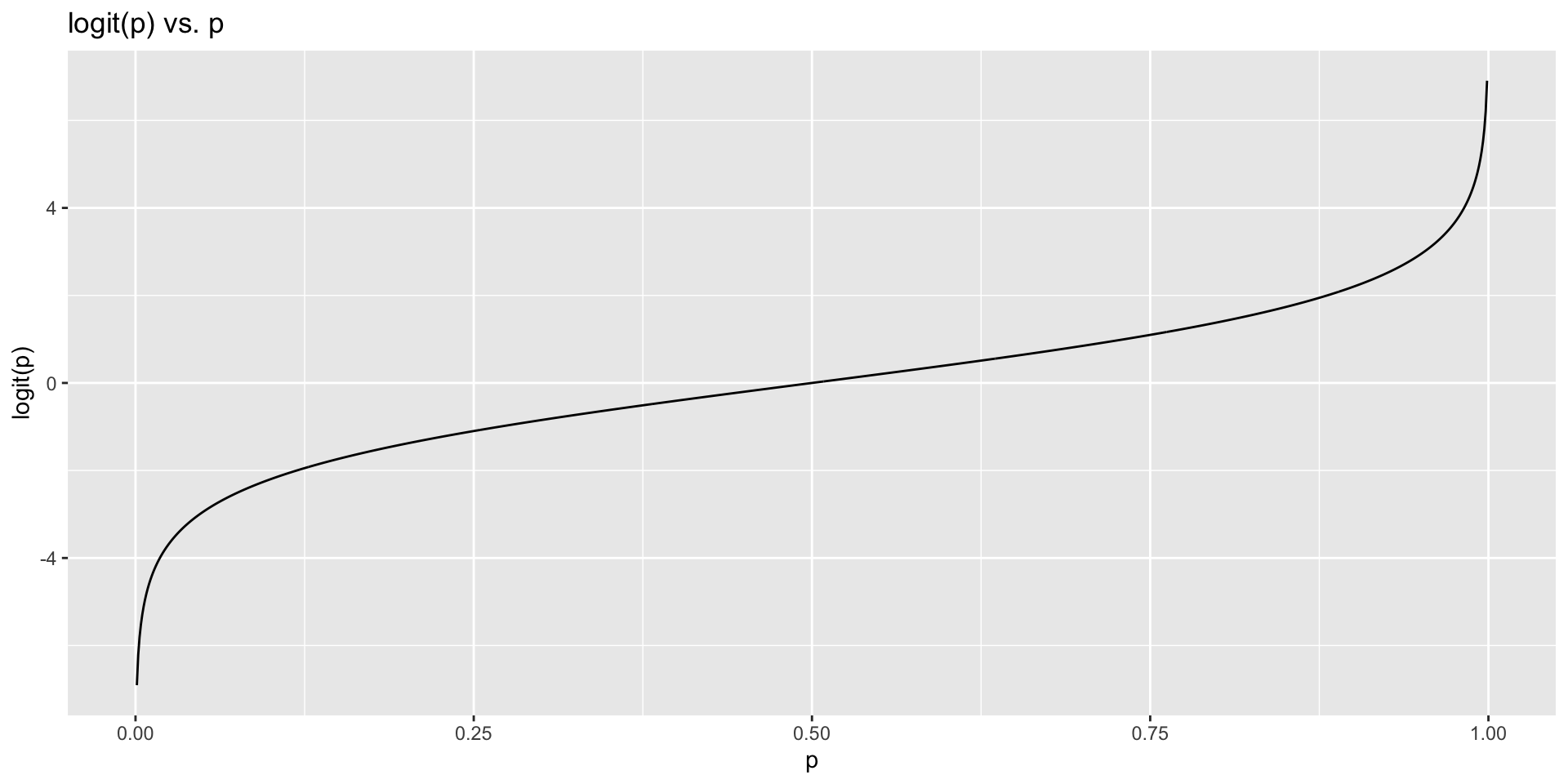
• In logistic regression, the link function that connects \(\eta_i\) to \(p_i\) is the logit function
• Logit function: For \(0\le p \le 1\)

\[logit(p) = \log\left(\frac{p}{1-p}\right)\]

Logit Function

Logistic Regression Model

• \(y_i \sim \text{Bern}(p_i)\)
• \(\eta_i = \beta_0+ \beta_1 x_{1,i} + \cdots + \beta_n x_{n,i}\)
• \(\text{logit}(p_i) = \eta_i\)

Logistic Regression Model

• \(\text{logit}(p_i) = \eta_i = \beta_0+ \beta_1 x_{1,i} + \cdots + \beta_n x_{n,i}\)
• Now take inverse logit to get \(p\)

\[p_i = \frac{\exp(\beta_0+\beta_1 x_{1,i} + \cdots + \beta_k x_{k,i})}{1+\exp(\beta_0+\beta_1 x_{1,i} + \cdots + \beta_k x_{k,i})}\]

A Worked Example

\[\log\left(\frac{p}{1-p}\right) = -1.16 - 0.33 \times \text{logGDPpc}\]

Country	logGDPpc	Linear predictor \(\eta\)	Odds	Probability \(p\)
Poor	6	\(-3.14\)	\(0.043\)	\(0.041\)
Middle	8	\(-3.80\)	\(0.022\)	\(0.022\)
Rich	10	\(-4.46\)	\(0.012\)	\(0.011\)

• The linear predictor \(\eta\) is unbounded — it can be any value
• The logit link keeps the predicted probability between 0 and 1
• Conflict onset is rare — small probabilities make sense

Analyzing Conflict Onset

The peacesciencer Package

• The peacesciencer package provides a number of datasets and functions for analyzing conflict and peace
• Provides data from a number of important datasets in the field of conflict studies, e.g.
  • Correlates of War (CoW) project
  • Uppsala Conflict Data Program (UCDP)
  • Militarized Interstate Dispute (MID) dataset
• Provides functions for analyzing conflict and adding control variables to the dataset

Using the peacesciencer Package

library(peacesciencer)

conflict_df <- create_stateyears(system = 'gw') |>
  filter(year %in% c(1946:1999)) |>
  add_ucdp_acd(type=c("intrastate"), only_wars = FALSE) |>
  add_democracy() |>
  add_creg_fractionalization() |>
  add_sdp_gdp() |>
  add_rugged_terrain()

glimpse(conflict_df)

Rows: 7,624
Columns: 22
$ gwcode         <dbl> 2, 2, 2, 2, 2, 2, 2, 2, 2, 2, 2, 2, 2, 2, 2, 2, 2, 2, 2…
$ gw_name        <chr> "United States of America", "United States of America",…
$ microstate     <dbl> 0, 0, 0, 0, 0, 0, 0, 0, 0, 0, 0, 0, 0, 0, 0, 0, 0, 0, 0…
$ year           <dbl> 1946, 1947, 1948, 1949, 1950, 1951, 1952, 1953, 1954, 1…
$ ucdpongoing    <dbl> 0, 0, 0, 0, 0, 0, 0, 0, 0, 0, 0, 0, 0, 0, 0, 0, 0, 0, 0…
$ ucdponset      <dbl> 0, 0, 0, 0, 0, 0, 0, 0, 0, 0, 0, 0, 0, 0, 0, 0, 0, 0, 0…
$ maxintensity   <dbl> NA, NA, NA, NA, NA, NA, NA, NA, NA, NA, NA, NA, NA, NA,…
$ conflict_ids   <chr> NA, NA, NA, NA, NA, NA, NA, NA, NA, NA, NA, NA, NA, NA,…
$ euds           <dbl> 1.293985, 1.308359, 1.343539, 1.330836, 1.354015, 1.350…
$ aeuds          <dbl> 0.4862558, 0.5006298, 0.5358093, 0.5231064, 0.5462858, …
$ polity2        <dbl> 9, 9, 9, 9, 9, 9, 9, 9, 9, 9, 9, 9, 9, 9, 9, 9, 9, 9, 9…
$ v2x_polyarchy  <dbl> 0.603, 0.607, 0.599, 0.580, 0.585, 0.611, 0.611, 0.612,…
$ ethfrac        <dbl> 0.2226323, 0.2248701, 0.2271561, 0.2294918, 0.2318781, …
$ ethpol         <dbl> 0.4152487, 0.4186156, 0.4220368, 0.4255134, 0.4290458, …
$ relfrac        <dbl> 0.4980802, 0.5009111, 0.5037278, 0.5065309, 0.5093204, …
$ relpol         <dbl> 0.7769888, 0.7770017, 0.7770303, 0.7770729, 0.7771274, …
$ wbgdp2011est   <dbl> 28.539, 28.519, 28.545, 28.534, 28.572, 28.635, 28.669,…
$ wbpopest       <dbl> 18.744, 18.756, 18.781, 18.804, 18.821, 18.832, 18.848,…
$ sdpest         <dbl> 28.478, 28.456, 28.483, 28.469, 28.510, 28.576, 28.611,…
$ wbgdppc2011est <dbl> 9.794, 9.762, 9.764, 9.730, 9.752, 9.803, 9.821, 9.857,…
$ rugged         <dbl> 1.073, 1.073, 1.073, 1.073, 1.073, 1.073, 1.073, 1.073,…
$ newlmtnest     <dbl> 3.214868, 3.214868, 3.214868, 3.214868, 3.214868, 3.214…

Running a Logistic Regression

• Implementation is not very different from a linear model
• Instead of lm(), we use glm() with family = "binomial"
• The family argument specifies the logit link function automatically

Bivariate Logistic Regression

conflict_model <- glm(ucdponset ~ wbgdppc2011est,
                      data = conflict_df,
                      family = "binomial")

summary(conflict_model)

Call:
glm(formula = ucdponset ~ wbgdppc2011est, family = "binomial", 
    data = conflict_df)

Coefficients:
               Estimate Std. Error z value Pr(>|z|)    
(Intercept)    -1.00735    0.41297  -2.439   0.0147 *  
wbgdppc2011est -0.35695    0.05089  -7.015 2.31e-12 ***
---
Signif. codes:  0 '***' 0.001 '**' 0.01 '*' 0.05 '.' 0.1 ' ' 1

(Dispersion parameter for binomial family taken to be 1)

    Null deviance: 1420.5  on 7623  degrees of freedom
Residual deviance: 1381.9  on 7622  degrees of freedom
AIC: 1385.9

Number of Fisher Scoring iterations: 7

Your Turn!

• Run a bivariate logistic regression using ucdponset as the outcome variable
• Try a different predictor (e.g., v2x_polyarchy, ethfrac, rugged)
• Examine the model output with summary()
• What direction is the effect? Is it significant?