Outliers and Model Assumptions

August 24, 2026

Dealing with Outliers

What Are Outliers?

Observations that don’t fit the general pattern of the data
Not always errors — often substantively interesting cases
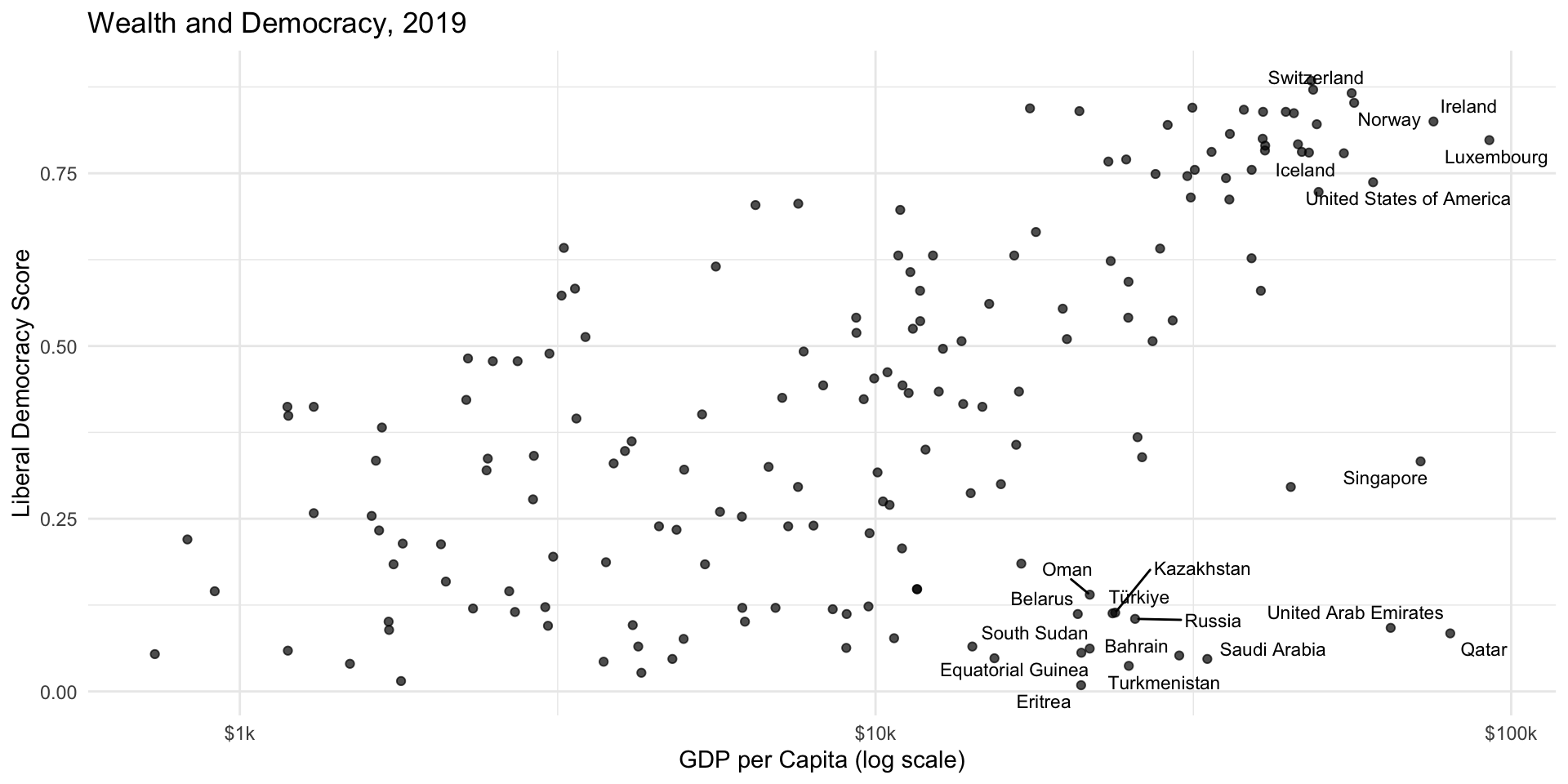
In our GDP-democracy example: oil-rich authoritarian states

Three Types of Outliers

Leverage points: extreme values on the x-axis
- Unusual predictor values; potential to distort the model
Influential points: significantly change the regression line when removed
- Combine extreme predictors and large residuals
Residual outliers: points far from the regression line
- Poorly fit by the model, regardless of their x-value

Revisiting Our GDP-Democracy Data

Identifying Outliers: IQR Method

Code

library(patchwork)

p1 <- ggplot(model_data, aes(y = lib_dem)) +
  geom_boxplot() +
  labs(y = "Liberal Democracy Score", title = "Democracy") +
  theme_minimal()

p2 <- ggplot(model_data, aes(y = wealth)) +
  geom_boxplot() +
  scale_y_continuous(labels = scales::dollar_format()) +
  labs(y = "GDP per Capita", title = "GDP (Raw)") +
  theme_minimal()

p1 | p2

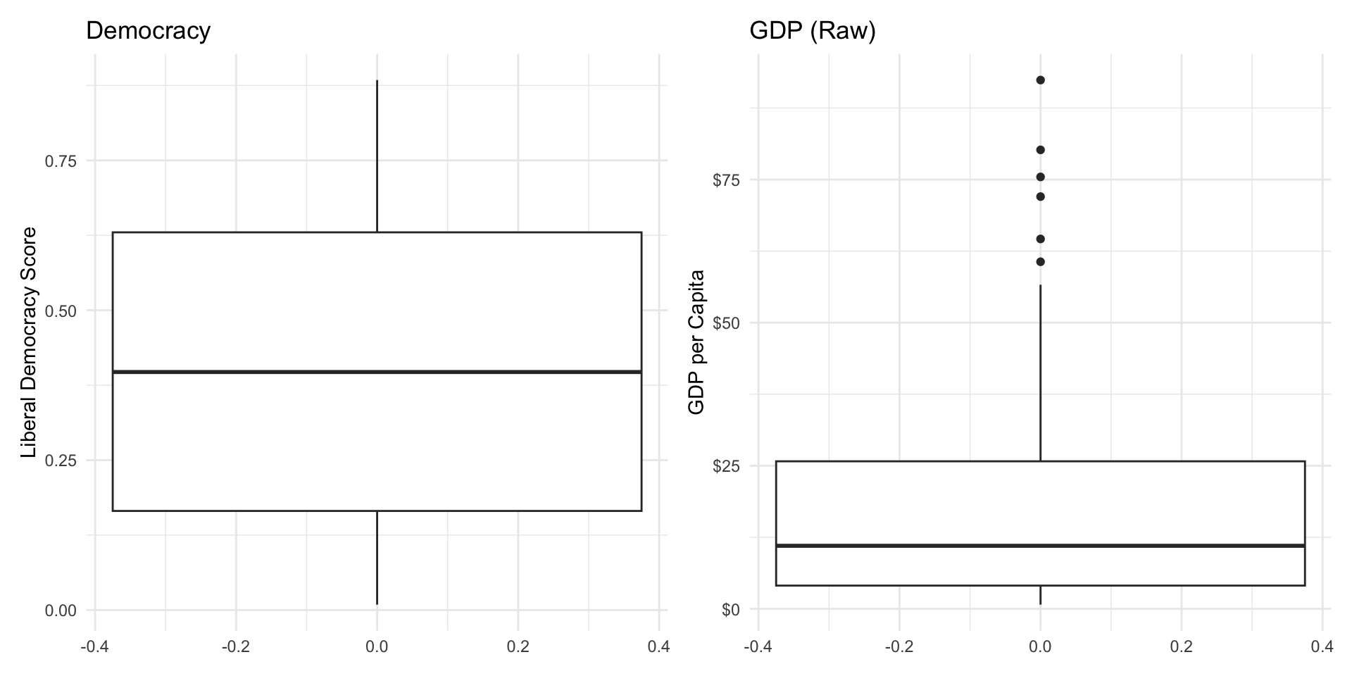
Flagging GDP Outliers

model_data <- model_data |>
  mutate(gdp_outlier = wealth %in% boxplot.stats(wealth)$out)

model_data |>
  filter(gdp_outlier) |>
  arrange(desc(wealth)) |>
  select(country, wealth, lib_dem)

                   country wealth lib_dem
1               Luxembourg 92.389   0.798
2                    Qatar 80.190   0.084
3                  Ireland 75.467   0.825
4                Singapore 72.025   0.333
5     United Arab Emirates 64.628   0.092
6 United States of America 60.641   0.737

Regression Diagnostics

The broom::augment() function adds diagnostic columns to our data:

Column	What it measures
`.hat`	Leverage — how extreme the predictor values are
`.std.resid`	Standardized residuals — how far from the line
`.cooksd`	Cook’s distance — overall influence on the model

Flagging Influential Points

democracy_model <- lm(lib_dem ~ log(wealth), data = model_data)

model_diagnostics <- augment(democracy_model, data = model_data) |>
  mutate(
    high_leverage  = .hat > 2 * mean(.hat),
    high_residual  = abs(.std.resid) > 2,
    high_influence = .cooksd > 4 / nrow(model_data)
  )

model_diagnostics |>
  filter(high_leverage | high_residual | high_influence) |>
  select(country, wealth, lib_dem, high_leverage, high_residual, high_influence)

# A tibble: 16 × 6
   country             wealth lib_dem high_leverage high_residual high_influence
   <chr>                <dbl>   <dbl> <lgl>         <lgl>         <lgl>         
 1 Venezuela            1.19    0.059 TRUE          FALSE         FALSE         
 2 Niger                1.19    0.399 TRUE          FALSE         FALSE         
 3 Burundi              0.735   0.054 TRUE          FALSE         FALSE         
 4 Central African Re…  0.827   0.22  TRUE          FALSE         FALSE         
 5 Ireland             75.5     0.825 TRUE          FALSE         FALSE         
 6 Liberia              1.19    0.412 TRUE          FALSE         FALSE         
 7 Malawi               1.31    0.412 TRUE          FALSE         FALSE         
 8 Qatar               80.2     0.084 TRUE          TRUE          TRUE          
 9 Democratic Republi…  0.913   0.145 TRUE          FALSE         FALSE         
10 Eritrea             21.1     0.009 FALSE         TRUE          FALSE         
11 Madagascar           1.31    0.258 TRUE          FALSE         FALSE         
12 Turkmenistan        25.0     0.037 FALSE         TRUE          FALSE         
13 Bahrain             30.0     0.052 FALSE         TRUE          TRUE          
14 Luxembourg          92.4     0.798 TRUE          FALSE         FALSE         
15 Saudi Arabia        33.3     0.047 FALSE         TRUE          TRUE          
16 United Arab Emirat… 64.6     0.092 FALSE         TRUE          TRUE

Your Turn!

Run the model using polarization as the predictor instead of wealth
Use augment() to identify influential observations in this new model
What countries stand out? Are they the same as in the GDP model?

Outlier Strategies

Four Main Strategies

Leave them in — outliers may be substantively important
Remove them — check how much they change your results
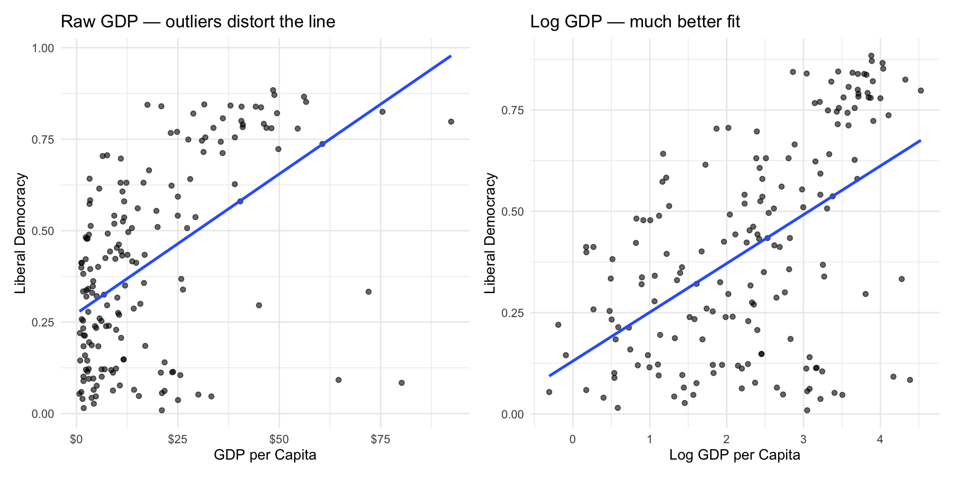
Transform the data — e.g., log transformation compresses extreme values
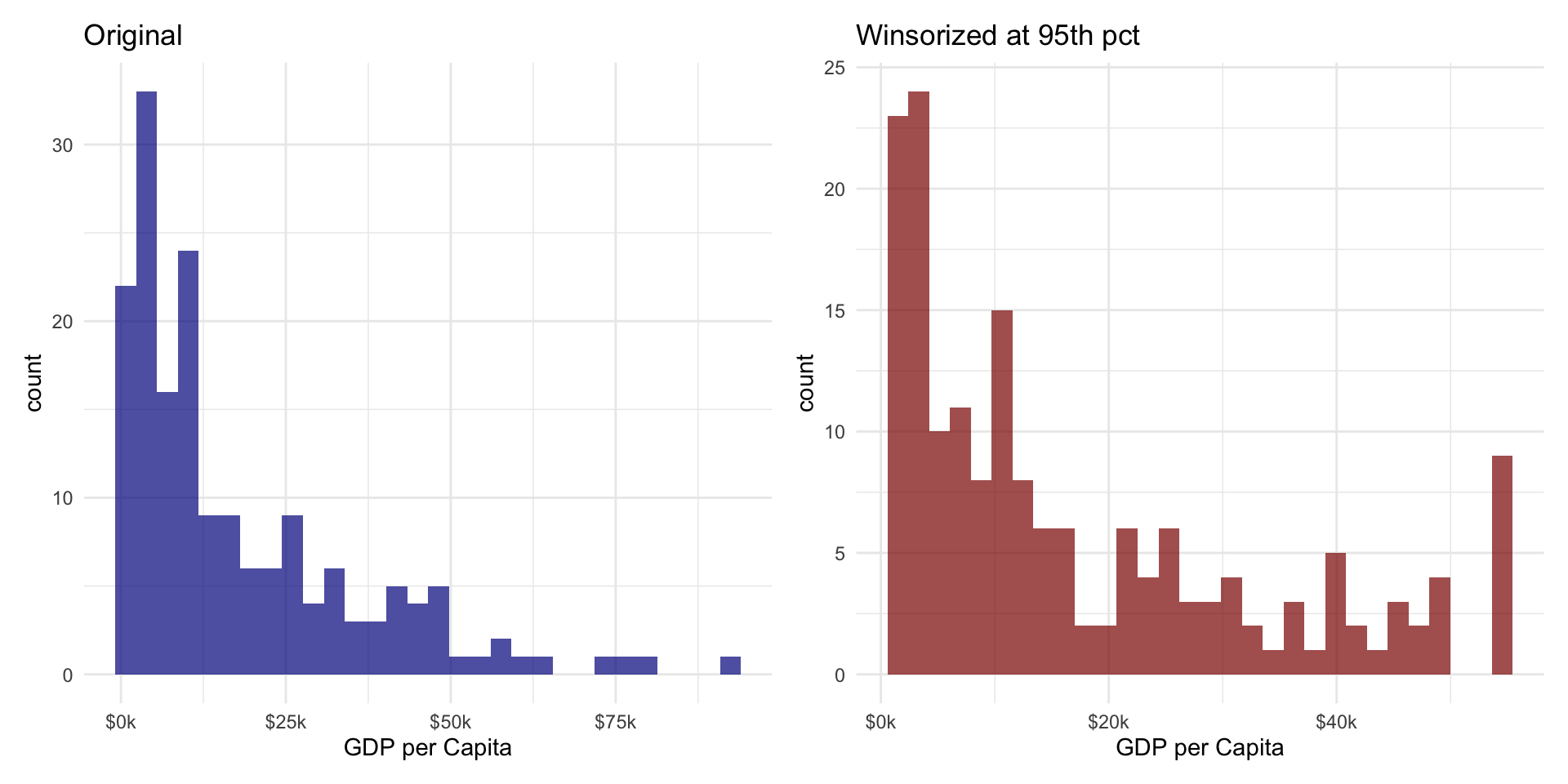
Winsorize — cap extreme values at a percentile rather than removing them

Strategy 1: Removing Outliers

Compare models with and without influential points:

# Original model
model_full <- lm(lib_dem ~ log(wealth), data = model_data)

# Model without influential points
model_data_clean <- model_diagnostics |>
  filter(!high_leverage & !high_residual & !high_influence)

model_clean <- lm(lib_dem ~ log(wealth), data = model_data_clean)

# Compare coefficients
tibble(
  model = c("Full", "No outliers"),
  intercept = c(coef(model_full)[1], coef(model_clean)[1]),
  slope = c(coef(model_full)[2], coef(model_clean)[2]),
  r_squared = c(glance(model_full)$r.squared, glance(model_clean)$r.squared)
)

# A tibble: 2 × 4
  model       intercept slope r_squared
  <chr>           <dbl> <dbl>     <dbl>
1 Full           0.131  0.120     0.280
2 No outliers    0.0693 0.152     0.372

Strategy 2: Log Transformation

Strategy 3: Winsorizing

Winsorizing caps extreme values at a specified percentile instead of removing them:

Code

library(datawizard)

model_data_win <- model_data |>
  mutate(wealth_win95 = winsorize(wealth, threshold = 0.05))

p1 <- ggplot(model_data, aes(x = wealth)) +
  geom_histogram(bins = 30, fill = "darkblue", alpha = 0.7) +
  scale_x_continuous(labels = scales::label_dollar(suffix = "k")) +
  labs(title = "Original", x = "GDP per Capita") +
  theme_minimal()

p2 <- ggplot(model_data_win, aes(x = wealth_win95)) +
  geom_histogram(bins = 30, fill = "darkred", alpha = 0.7) +
  scale_x_continuous(labels = scales::label_dollar(suffix = "k")) +
  labs(title = "Winsorized at 95th pct", x = "GDP per Capita") +
  theme_minimal()

p1 | p2

Strategy 4: Robust Regression

MASS::rlm() is less sensitive to outliers than OLS:

library(MASS)

robust_model <- rlm(lib_dem ~ log(wealth), data = model_data)

summary(robust_model)


Call: rlm(formula = lib_dem ~ log(wealth), data = model_data)
Residuals:
     Min       1Q   Median       3Q      Max 
-0.60880 -0.15368  0.03422  0.17024  0.37024 

Coefficients:
            Value  Std. Error t value
(Intercept) 0.1178 0.0385     3.0619 
log(wealth) 0.1311 0.0149     8.8195 

Residual standard error: 0.2429 on 172 degrees of freedom

How to Choose?

Situation	Strategy
Data entry error or wrong population	Remove
Naturally skewed variable	Log transform
Want to keep all obs., reduce tail influence	Winsorize
Outliers are legitimate but numerous	Robust regression
Outliers are theoretically interesting	Leave in; discuss

Note

Always report your decision and run a sensitivity analysis to show how results change.

Your Turn!

Go back to the polarization model you built earlier
Try removing the influential points and compare to the original model
Now try winsorizing polarization at the 95th percentile
Which approach changes the results more?

Checking Model Assumptions (Optional)

Why Check Assumptions?

Linear regression makes several assumptions about your data
Violating them can lead to biased coefficients or wrong standard errors
Checking assumptions helps you know when to trust your results

The LINE Conditions

Letter	Assumption	What it means
L	Linearity	Relationship between X and Y is linear
I	Independence	Observations are independent of each other
N	Normality	Residuals are approximately normally distributed
E	Equal variance	Residuals have constant variance (homoscedasticity)

Setup for Diagnostics

library(vdemlite)

model_data2 <- fetchdem(
  indicators = c("v2x_libdem", "e_gdppc", "v2cacamps",
                 "v2x_gender", "v2x_corr", "e_regionpol_6C"),
  start_year = 2006, end_year = 2006
) |>
  rename(country = country_name, lib_dem = v2x_libdem,
         wealth = e_gdppc, polarization = v2cacamps,
         women_emp = v2x_gender, corruption = v2x_corr,
         region = e_regionpol_6C) |>
  mutate(region = factor(region,
    labels = c("Eastern Europe", "Latin America", "MENA",
               "SS Africa", "The West", "Asia & Pacific")))

democracy_model2 <- lm(lib_dem ~ log(wealth) + polarization +
                         corruption + women_emp + region,
                       data = model_data2)

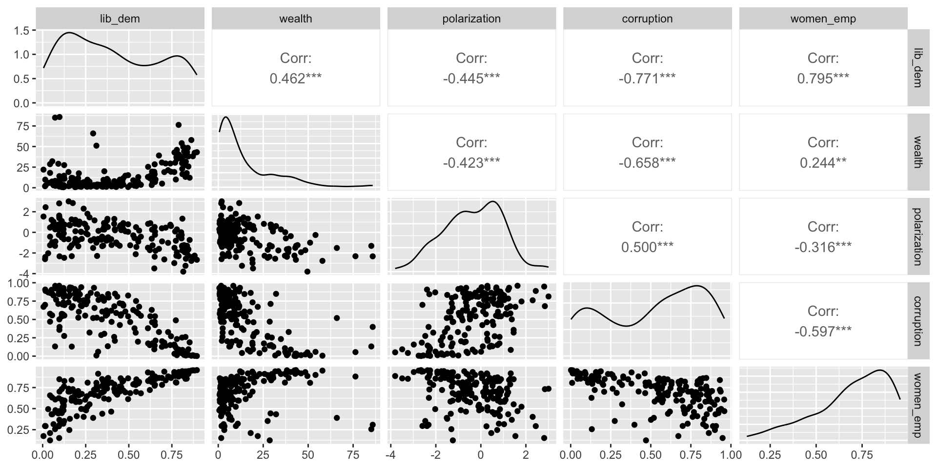
Exploratory Data Analysis First

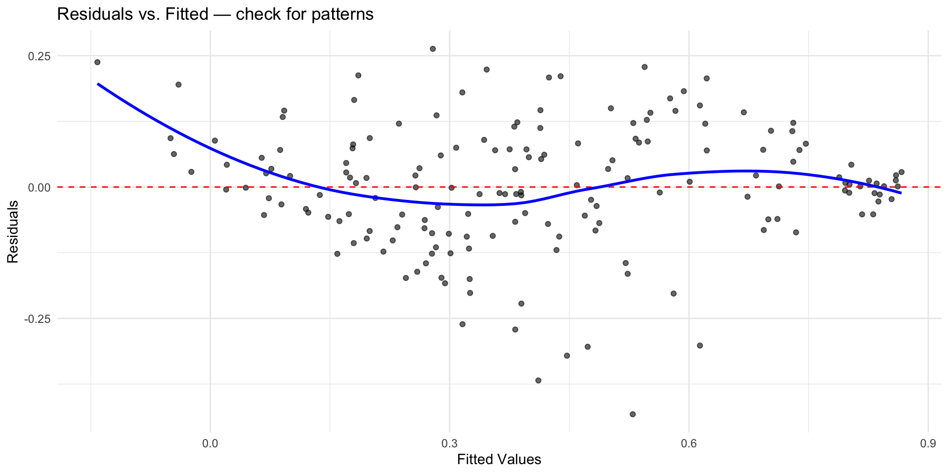
Checking Linearity: Residuals vs. Fitted

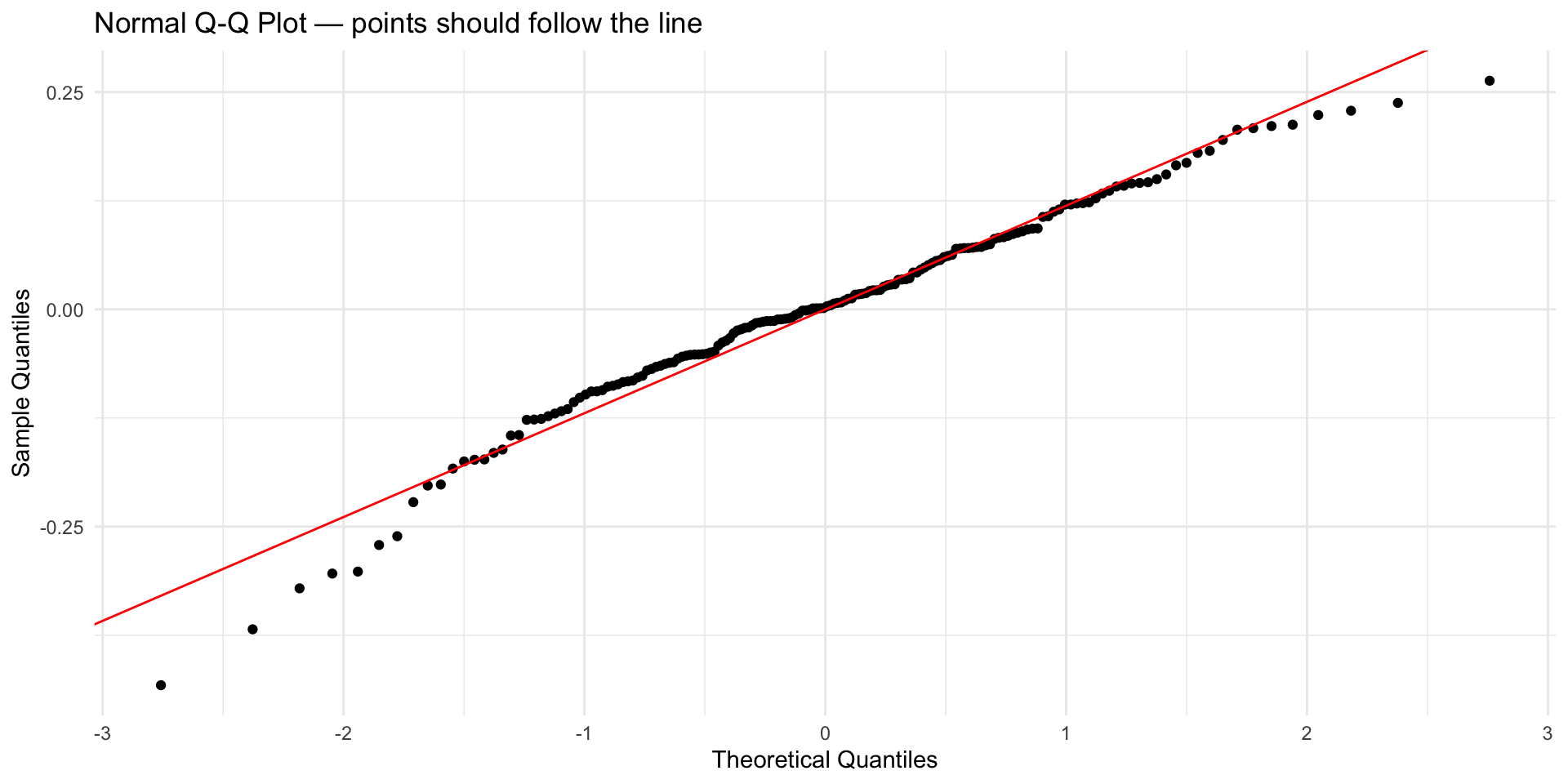
Checking Normality: Q-Q Plot

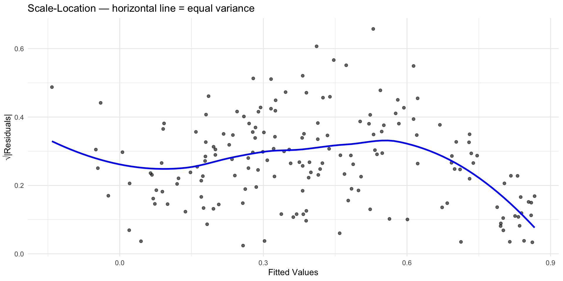
Checking Equal Variance: Scale-Location

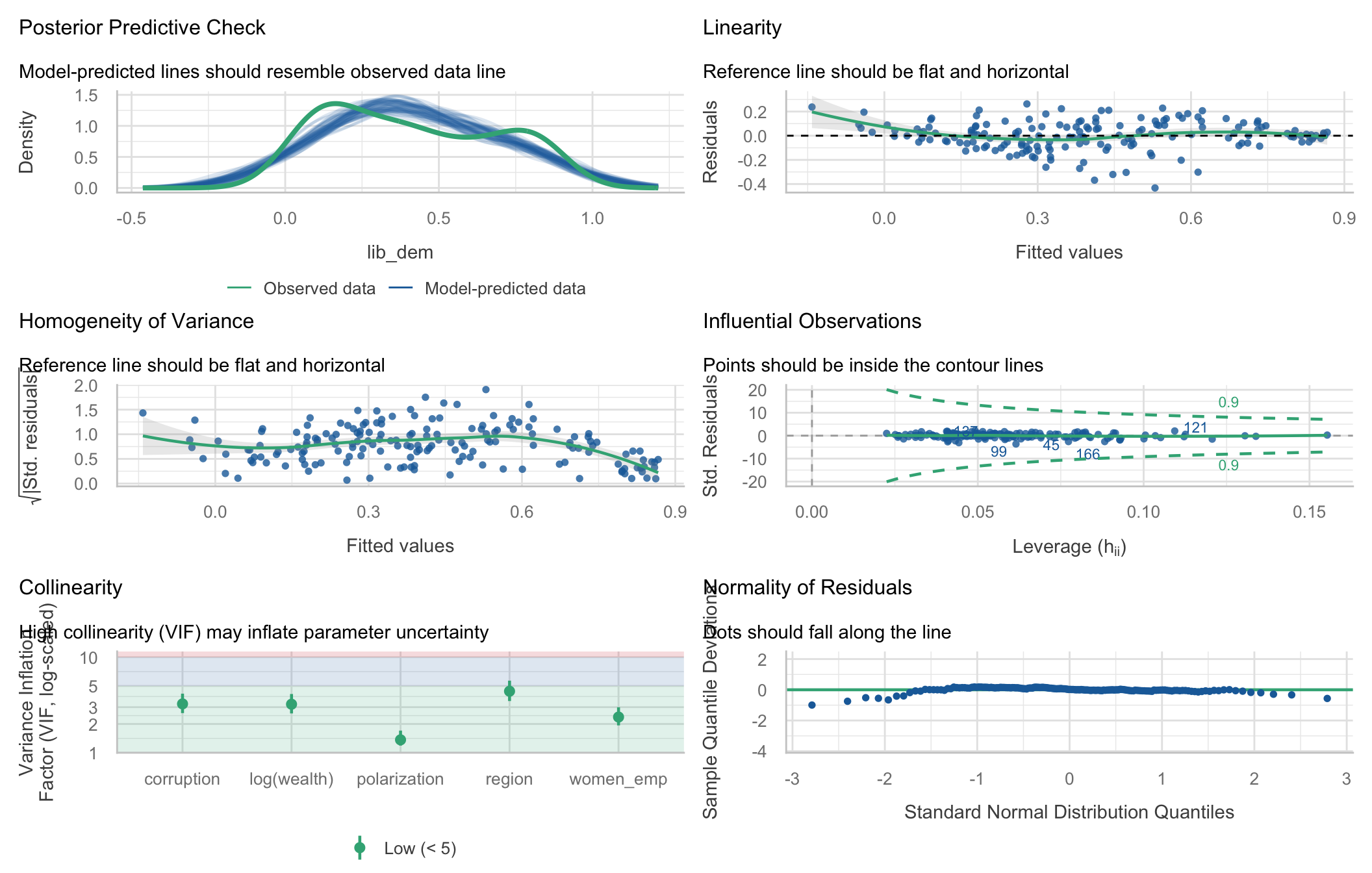
Automated Diagnostics with `performance`

You can automate all the diagnostics we just discussed with a single line of code using the performance package:

library(performance)

check_model(democracy_model2)

Fixing Violations: Transformations

If you detect assumption violations:

Log transform skewed predictors → compresses extremes, improves linearity
Polynomial terms → capture curved relationships: I(x^2)
Robust standard errors → correct inference under heteroscedasticity

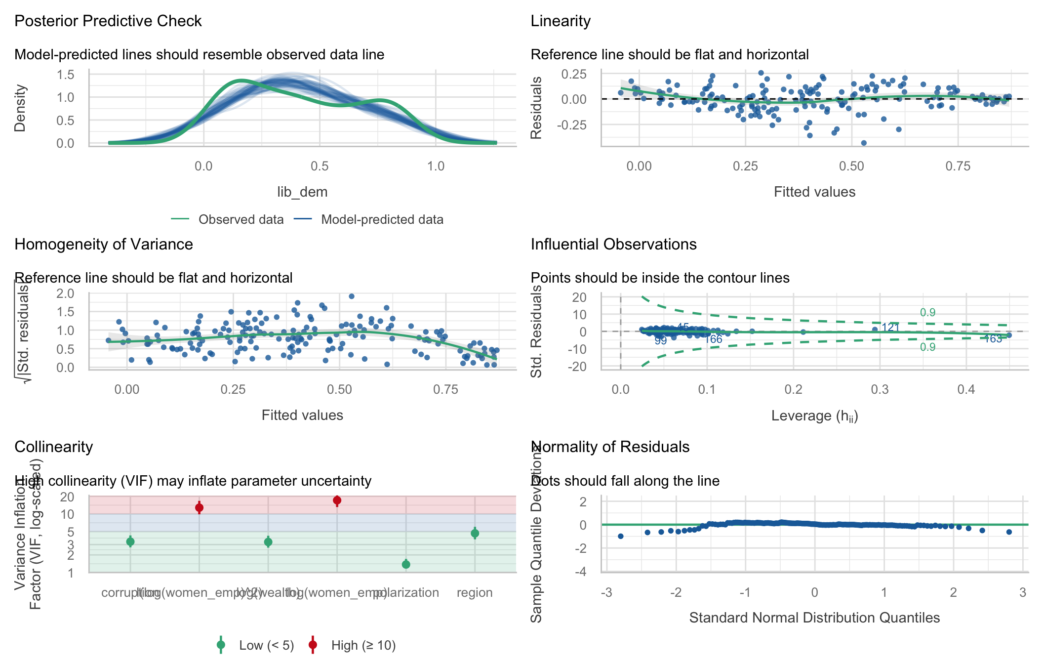
Example: Addressing Non-Linearity

Adding a polynomial term for women_emp to capture a curved relationship:

democracy_model3 <- lm(
  lib_dem ~ log(wealth) + polarization + corruption +
    log(women_emp) + I(log(women_emp)^2) + region,
  data = model_data2
)

check_model(democracy_model3)

Your Turn!

Run check_model() on a model from your own project
Which LINE assumptions look satisfied? Which look violated?
Try a log transformation on a skewed predictor — does it improve the diagnostics?

Outliers and Model Assumptions

Dealing with Outliers

What Are Outliers?

Three Types of Outliers

Revisiting Our GDP-Democracy Data

Identifying Outliers: IQR Method

Flagging GDP Outliers

Regression Diagnostics

Flagging Influential Points

Your Turn!

Outlier Strategies

Four Main Strategies

Strategy 1: Removing Outliers

Strategy 2: Log Transformation

Strategy 3: Winsorizing

Strategy 4: Robust Regression

How to Choose?

Your Turn!

Checking Model Assumptions (Optional)

Why Check Assumptions?

The LINE Conditions

Setup for Diagnostics

Exploratory Data Analysis First

Checking Linearity: Residuals vs. Fitted

Checking Normality: Q-Q Plot

Checking Equal Variance: Scale-Location

Automated Diagnostics with performance

Fixing Violations: Transformations

Example: Addressing Non-Linearity

Your Turn!

Automated Diagnostics with `performance`