Multiple Regression
September 21, 2026
Load packages
Load VDEM Data
modelData <- vdem |>
  filter(year == 2006) |>
  select(country_name,
         libdem = v2x_libdem,
         wealth = e_gdppc,
         oil_rents = e_total_oil_income_pc,
         polarization = v2cacamps,
         corruption = v2x_corr,
         judicial_review = v2jureview_ord,
         region = e_regionpol_6C,
         regime = v2x_regime) |>
  mutate(log_wealth = log(wealth),
         region = factor(
           region,
           labels=c("Eastern Europe",
             "Latin America",
             "MENA",
             "SSAfrica",
             "Western Europe and North America",
             "Asia and Pacific"))
          )

glimpse(modelData)
Rows: 177
Columns: 10
$ country_name <chr> "Mexico", "Suriname", "Sweden", "Switzerland", "Ghana"…
$ libdem <dbl> 0.478, 0.649, 0.879, 0.841, 0.634, 0.661, 0.773, 0.018…
$ wealth <dbl> 31.873, 22.316, 98.394, 105.485, 6.471, 23.398, 84.983…
$ oil_rents <dbl> 694.847, 639.506, 0.000, 0.000, 6.380, 10.060, 2.635, …
$ polarization <dbl> 0.035, -1.815, -2.283, -1.767, -0.500, 0.006, -2.269, …
$ corruption <dbl> 0.609, 0.199, 0.004, 0.023, 0.625, 0.444, 0.108, 0.878…
$ judicial_review <dbl> 1, 1, 1, 1, 1, 1, 1, 0, 1, 1, 1, 0, 1, 1, 1, 1, 1, 1, …
$ region <fct> Latin America, Latin America, Western Europe and North…
$ regime <dbl> 2, 2, 3, 3, 3, 3, 3, 0, 1, 2, 1, 1, 2, 3, 2, 3, 3, 2, …
$ log_wealth <dbl> 3.461759, 3.105304, 4.588980, 4.658569, 1.867331, 3.15…Linear Model with Multiple Predictors
- Previously, we were interested in GDP per capita as a predictor of democracy
- Now, let’s consider another predictor: polarization (also measured by V-Dem)
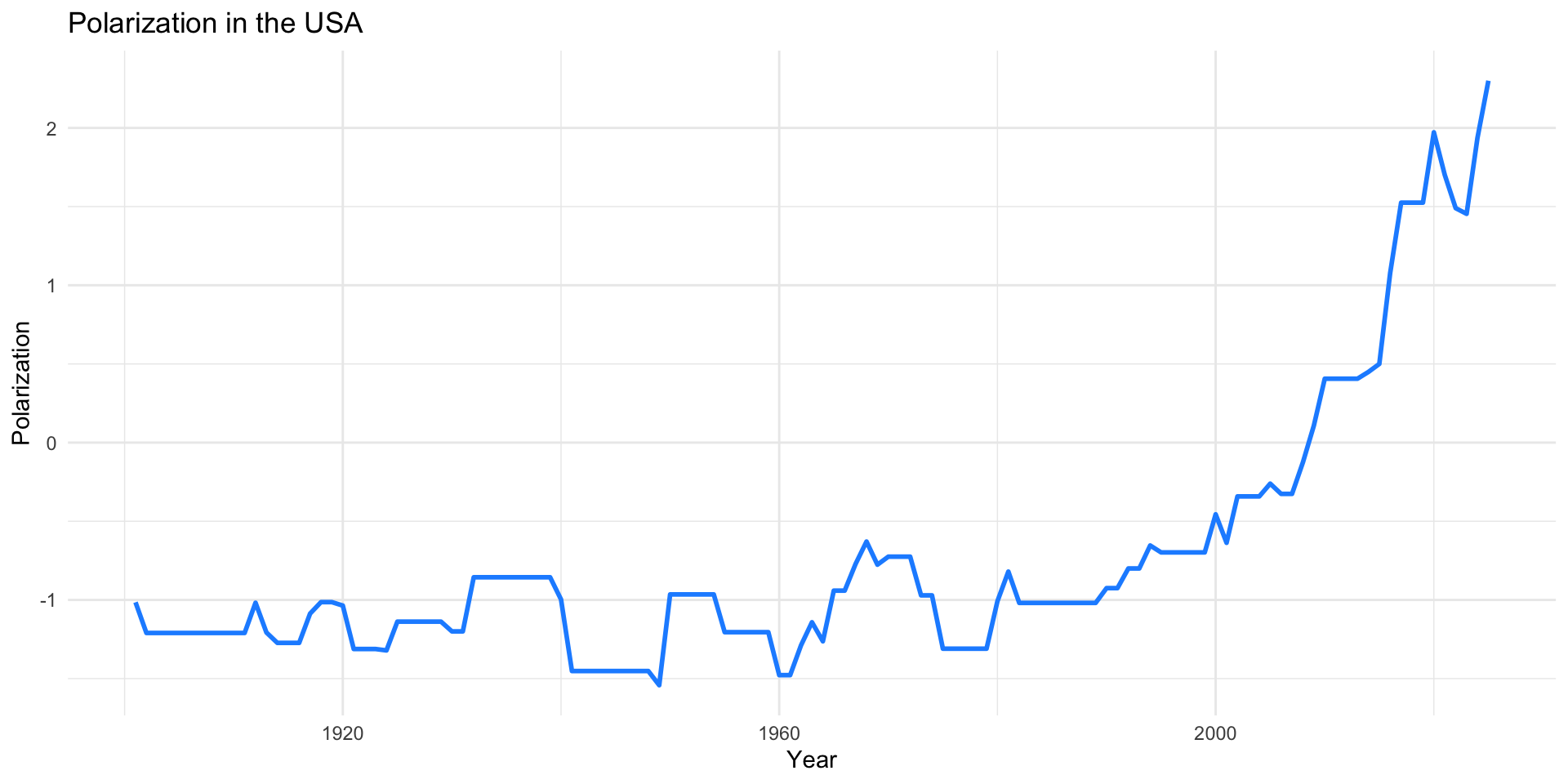
Polarization Measure in the USA
Polarization and Democracy in 2006
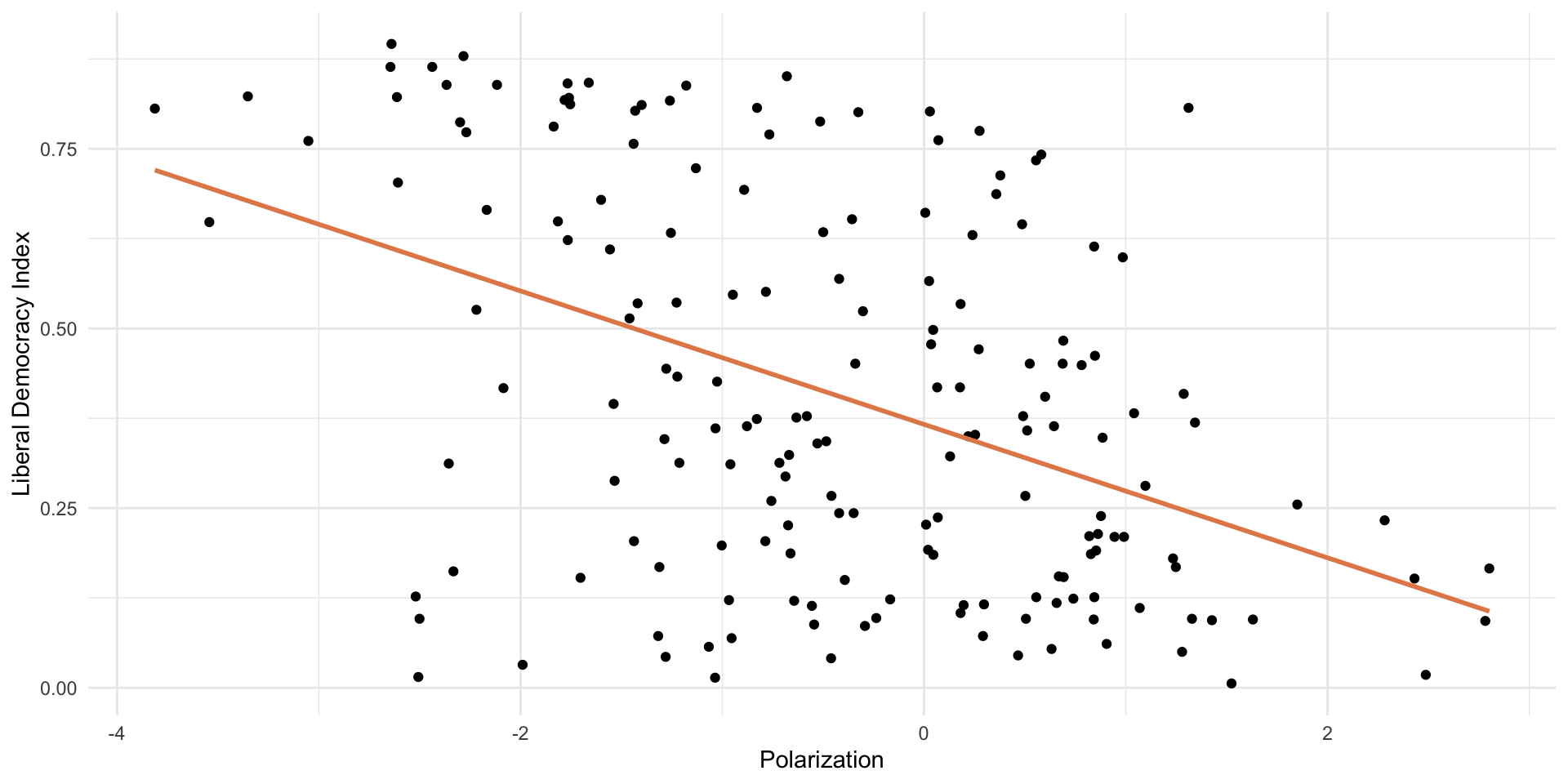
Model with One Predictor
Call:
lm(formula = libdem ~ polarization, data = modelData)

Residuals:
     Min       1Q   Median       3Q      Max
-0.58420 -0.17264 -0.03252  0.18056  0.56220

Coefficients:
             Estimate Std. Error t value Pr(>|t|)
(Intercept)   0.36649    0.01895   19.34  < 2e-16 ***
polarization -0.09282    0.01404   -6.61 4.47e-10 ***
---
Signif. codes:  0 '***' 0.001 '**' 0.01 '*' 0.05 '.' 0.1 ' ' 1

Residual standard error: 0.2398 on 175 degrees of freedom
Multiple R-squared:  0.1998,    Adjusted R-squared:  0.1952
F-statistic: 43.7 on 1 and 175 DF, p-value: 4.466e-10Significance?
Model with Two Predictors
Call:
lm(formula = libdem ~ polarization + log_wealth, data = modelData)

Residuals:
     Min       1Q   Median       3Q      Max
-0.66770 -0.15112  0.04516  0.17776  0.42283

Coefficients:
             Estimate Std. Error t value Pr(>|t|)
(Intercept)   0.09668    0.04423   2.186   0.0302 *
polarization -0.05779    0.01372  -4.213 4.08e-05 ***
log_wealth    0.09998    0.01495   6.687 3.14e-10 ***
---
Signif. codes:  0 '***' 0.001 '**' 0.01 '*' 0.05 '.' 0.1 ' ' 1

Residual standard error: 0.216 on 170 degrees of freedom
  (4 observations deleted due to missingness)
Multiple R-squared:  0.3656,    Adjusted R-squared:  0.3582
F-statistic: 48.99 on 2 and 170 DF,  p-value: < 2.2e-16
Model with Two Predictors
\[\hat{Y_i} = a + b_1*Polarization + b_2*GDPpc\]
\[\hat{Y_i} = 0.10 + -0.06*Polarization + 0.10*GDPpc\]
Model with Two Predictors
\[\hat{Y_i} = a + b_1*Polarization + b_2*GDPpc\]
\[\hat{Y_i} = 0.10 + -0.06*Polarization + 0.10*GDPpc\]
\(a\) is the predicted level of Y when BOTH GDP per capita and polarization are equal to 0
Model with Two Predictors
\[\hat{Y_i} = a + b_1*Polarization + b_2*GDPpc\]
\[\hat{Y_i} = 0.10 + -0.06*Polarization + 0.10*GDPpc\]
- \(b_1\) is the impact of a 1-unit change in polarization on the predicted level of Y, holding GDP per capita fixed (all else equal)
- The relationship between polarization and democracy, controlling for wealth
Model with Two Predictors
\[\hat{Y_i} = a + b_1*Polarization + b_2*GDPpc\]
\[\hat{Y_i} = 0.10 + -0.06*Polarization + 0.10*GDPpc\]
- \(b_2\) is the impact of a 1-unit change in GDP per capita on the predicted level of Y, holding polarization fixed (all else equal)
- The relationship between wealth and democracy, controlling for polarization
Model with Two Predictors
\[\hat{Y_i} = a + b_1*Polarization + b_2*GDPpc\]
- OLS is searching for combination of \(a\), \(b_1\), and \(b_2\) that minimize sum of squared residuals
- Same logic as model with one predictor, just more complicated
Model with Three Predictors
\[\hat{Y_i} = a + b_1*Polarization + b_2*GDPpc + b_3*OilRents\]
Model with Three Predictors
Call:
lm(formula = libdem ~ polarization + log_wealth + oil_rents,
    data = modelData)

Residuals:
     Min       1Q   Median       3Q      Max
-0.53085 -0.14849  0.03728  0.12810  0.67727

Coefficients:
               Estimate Std. Error t value Pr(>|t|)
(Intercept)   2.320e-02  4.151e-02   0.559    0.577
polarization -5.660e-02  1.270e-02  -4.458 1.56e-05 ***
log_wealth    1.371e-01  1.471e-02   9.315  < 2e-16 ***
oil_rents    -4.169e-05  5.915e-06  -7.048 5.32e-11 ***
---
Signif. codes:  0 '***' 0.001 '**' 0.01 '*' 0.05 '.' 0.1 ' ' 1

Residual standard error: 0.1922 on 158 degrees of freedom
  (15 observations deleted due to missingness)
Multiple R-squared:  0.5099,    Adjusted R-squared:  0.5006
F-statistic: 54.79 on 3 and 158 DF,  p-value: < 2.2e-16
Model with Three Predictors
\[\hat{Y_i} = a + b_1*Polarization + b_2*GDPpc + b_3*OilRents\]
\[\hat{Y_i} = a + -.06*Polarization + .14*GDPpc + -.00004*OilRents\]
Your Turn!
- In the last session, you examined levels of democracy and corruption
- Now, let’s fit a multiple regression model predicting corruption with two predictors: democracy (libdem) and polarization (polarization)
- Then, interpret the coefficients
- Estimate a second multiple regression model that adds in GDP per capita (lg_gdppc)
- Interpret the coefficients
- What happens to the coefficients of the other variables when we add GDP per capita to the model?
- Why do you think this happens?
- Try adding in additional predictors if there is time
Model 1
Call:
lm(formula = corruption ~ libdem + polarization, data = modelData)

Residuals:
    Min      1Q  Median      3Q     Max
-0.5998 -0.1084  0.0103  0.1363  0.3594

Coefficients:
             Estimate Std. Error t value Pr(>|t|)
(Intercept)   0.85173    0.02652  32.114  < 2e-16 ***
libdem       -0.78150    0.05973 -13.085  < 2e-16 ***
polarization  0.04529    0.01240   3.652 0.000344 ***
---
Signif. codes:  0 '***' 0.001 '**' 0.01 '*' 0.05 '.' 0.1 ' ' 1

Residual standard error: 0.1895 on 174 degrees of freedom
Multiple R-squared:  0.6201,    Adjusted R-squared:  0.6157
F-statistic:   142 on 2 and 174 DF,  p-value: < 2.2e-16
Model 2 - Adding GDP per capita
Call:
lm(formula = corruption ~ libdem + polarization + log_wealth,
    data = modelData)

Residuals:
     Min       1Q   Median       3Q      Max
-0.48471 -0.09085 -0.00029  0.12225  0.33234

Coefficients:
             Estimate Std. Error t value Pr(>|t|)
(Intercept)   1.02846    0.03456  29.763  < 2e-16 ***
libdem       -0.60887    0.05910 -10.303  < 2e-16 ***
polarization  0.03030    0.01111   2.728  0.00705 **
log_wealth   -0.08685    0.01295  -6.708 2.85e-10 ***
---
Signif. codes:  0 '***' 0.001 '**' 0.01 '*' 0.05 '.' 0.1 ' ' 1

Residual standard error: 0.1664 on 169 degrees of freedom
  (4 observations deleted due to missingness)
Multiple R-squared:  0.7099,    Adjusted R-squared:  0.7048
F-statistic: 137.9 on 3 and 169 DF,  p-value: < 2.2e-16
Categorical Variables
Judicial Review and Democracy
Judicial Review:
- Do high courts (Supreme Court, Constitutional Court, etc) have the power to rule on whether laws or policies are constitutional/legal? (Yes or No)
- Dimension of Judicial Independence
Judicial Review and Democracy
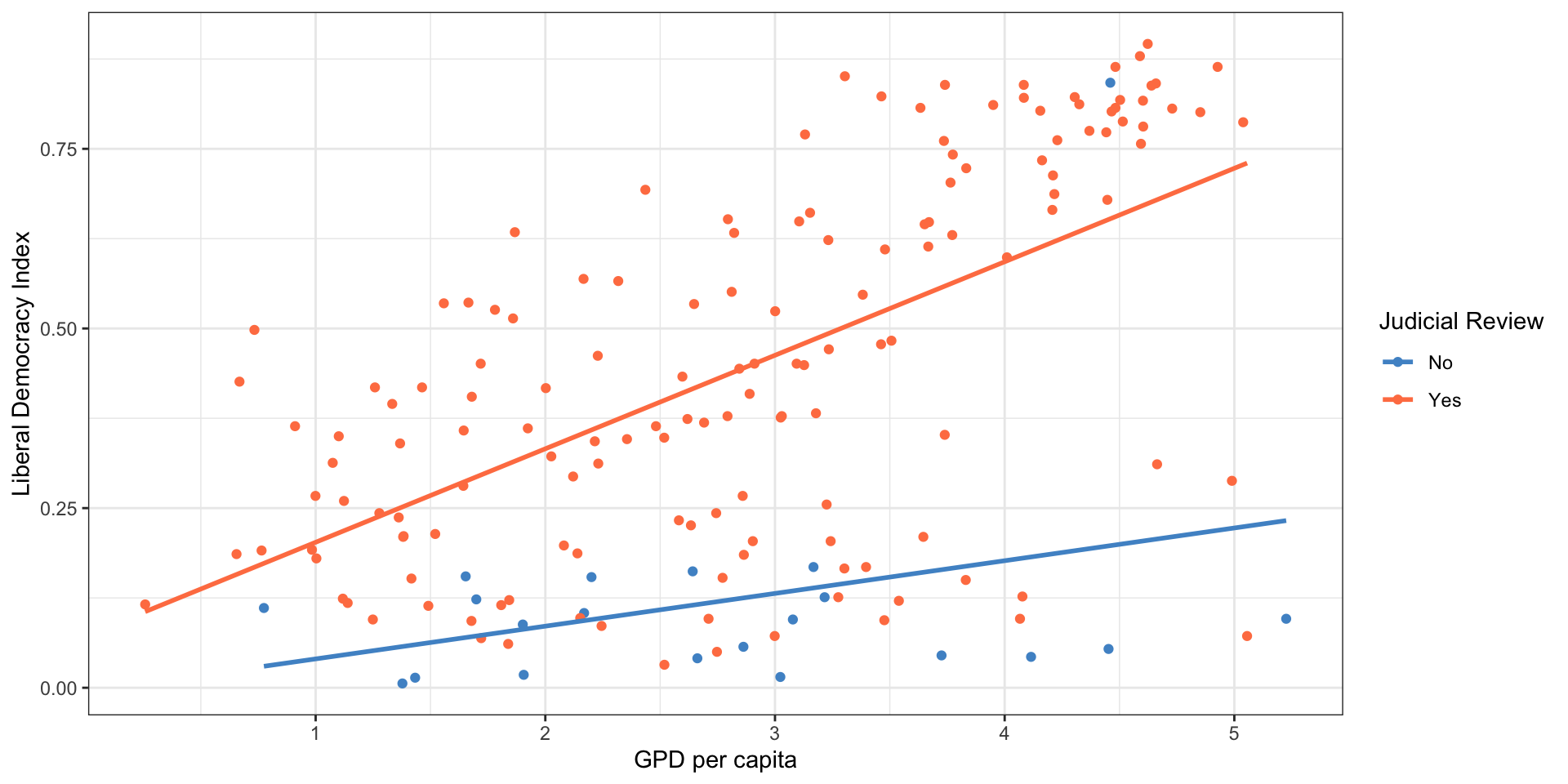
Judicial Review and Democracy
Call:
lm(formula = libdem ~ factor(judicial_review), data = modelData)

Residuals:
     Min       1Q   Median       3Q      Max
-0.41164 -0.20464 -0.03186  0.20436  0.72214

Coefficients:
                         Estimate Std. Error t value Pr(>|t|)
(Intercept)               0.11986    0.05380   2.228   0.0272 *
factor(judicial_review)1  0.32378    0.05731   5.650  6.4e-08 ***
---
Signif. codes:  0 '***' 0.001 '**' 0.01 '*' 0.05 '.' 0.1 ' ' 1

Residual standard error: 0.2466 on 175 degrees of freedom
Multiple R-squared:  0.1543,    Adjusted R-squared:  0.1494
F-statistic: 31.92 on 1 and 175 DF,  p-value: 6.403e-08
Judicial Review and Democracy
\[\widehat{Democracy_{i}} = 0.13 + 0.32*JudicialReview(yes)\]
- Slope: countries with judicial review are expected, on average, to be 0.32 units more democratic on the liberal democracy index
- Compares baseline level (Judicial Review = 0) to the other level (Judicial Review = 1)
- Intercept: average democracy score of countries without judicial review
- Average democracy score of countries with judicial review is 0.13 + 0.32 = 0.45
Dummy Variables
- When the categorical explanatory variable has many levels, they’re encoded to dummy variables
- We always leave one category out of the model, as the omitted reference category
- Each coefficient describes is the expected difference between level of the factor and the baseline level
- Everything is relative to the omitted reference category
Democracy and World Region
- Does region predict levels of democracy?
- Since Eastern Europe is the first category, default in R is to use that as the omitted category in models.
Democracy and World Region
How should we interpret intercept? How about the coefficient on Latin America?
Call:
lm(formula = libdem ~ region, data = modelData)

Residuals:
     Min       1Q   Median       3Q      Max
-0.45848 -0.13314 -0.02148  0.11452  0.49130

Coefficients:
                                       Estimate Std. Error t value Pr(>|t|)
(Intercept)                             0.43287    0.03598  12.030  < 2e-16 ***
regionLatin America                     0.06661    0.05337   1.248  0.21367
regionMENA                             -0.23717    0.05689  -4.169 4.86e-05 ***
regionSSAfrica                         -0.14065    0.04551  -3.090  0.00233 **
regionWestern Europe and North America  0.37343    0.05397   6.919 8.73e-11 ***
regionAsia and Pacific                 -0.13372    0.05179  -2.582  0.01065 *
---
Signif. codes:  0 '***' 0.001 '**' 0.01 '*' 0.05 '.' 0.1 ' ' 1

Residual standard error: 0.1971 on 171 degrees of freedom
Multiple R-squared:  0.472, Adjusted R-squared:  0.4566
F-statistic: 30.57 on 5 and 171 DF,  p-value: < 2.2e-16
Democracy and World Region
What if you want a different baseline category? How do we interpret now?
# make SS Africa the reference category
modelData <- modelData |>
mutate(newReg = relevel(region, ref=4))

lm(libdem ~ newReg, data = modelData) |> summary()
Call:
lm(formula = libdem ~ newReg, data = modelData)

Residuals:
     Min       1Q   Median       3Q      Max
-0.45848 -0.13314 -0.02148  0.11452  0.49130

Coefficients:
                                        Estimate Std. Error t value Pr(>|t|)
(Intercept)                             0.292220   0.027871  10.485  < 2e-16
newRegEastern Europe                    0.140647   0.045513   3.090  0.00233
newRegLatin America                     0.207260   0.048273   4.293 2.94e-05
newRegMENA                             -0.096520   0.052141  -1.851  0.06588
newRegWestern Europe and North America  0.514072   0.048939  10.504  < 2e-16
newRegAsia and Pacific                  0.006923   0.046517   0.149  0.88187

(Intercept)                            ***
newRegEastern Europe                   **
newRegLatin America                    ***
newRegMENA                             .
newRegWestern Europe and North America ***
newRegAsia and Pacific
---
Signif. codes:  0 '***' 0.001 '**' 0.01 '*' 0.05 '.' 0.1 ' ' 1

Residual standard error: 0.1971 on 171 degrees of freedom
Multiple R-squared:  0.472, Adjusted R-squared:  0.4566
F-statistic: 30.57 on 5 and 171 DF,  p-value: < 2.2e-16
Your Turn
Which types of regime have more corruption?
V-Dem also includes a categorial regime variable: Closed autocracy (0), Electoral Autocracy (1), Electoral Democracy (2), Liberal Democracy (3)
Your Turn
Which types of regime have more corruption?
First, let’s make this an easier factor variable to work with.
# Make nicer regime factor variable
modelData <- modelData |>
  mutate(regime = factor(regime,
                         labels = c("Closed Autocracy",
                                   "Electoral Autocracy",
                                  "Electoral Democracy",
                                  "Liberal Democracy")))
levels(modelData$regime)
[1] "Closed Autocracy" "Electoral Autocracy" "Electoral Democracy"
[4] "Liberal Democracy" Your Turn
Which types of regime have more corruption?
- Filter data to include only the year 2019 (or run the code to use modelData)
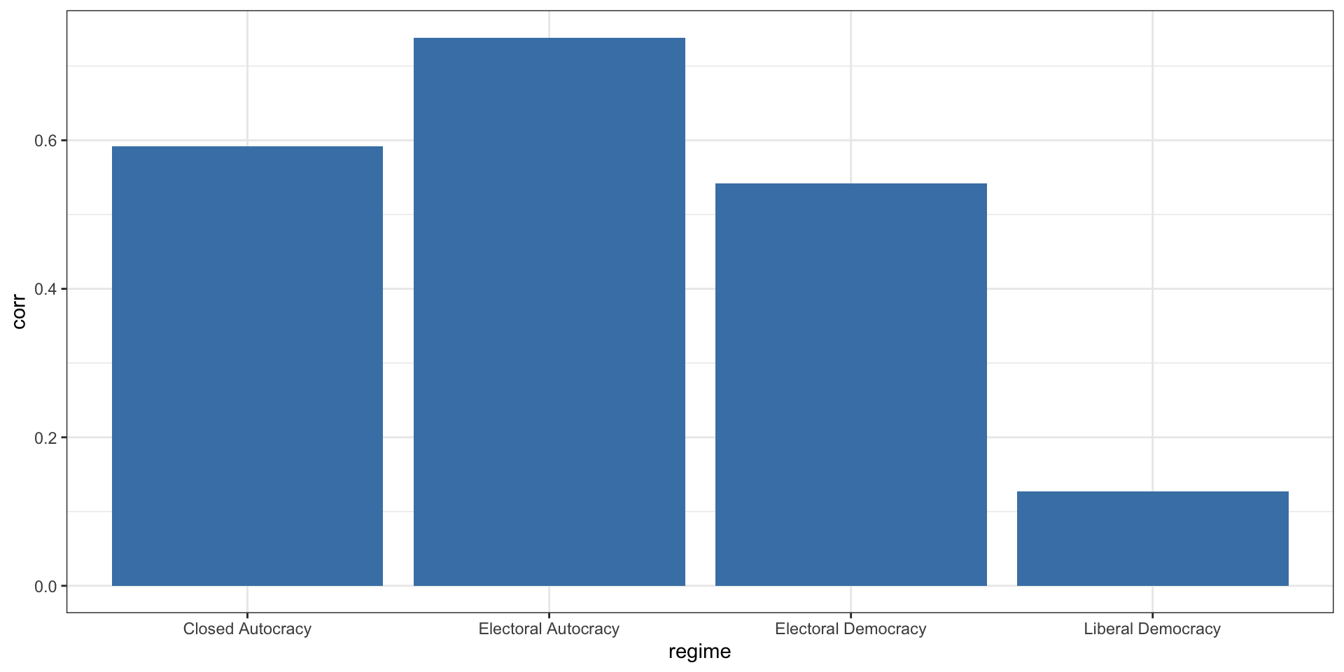
- Make a plot to visualize the relationship between regime type and level of corruption. - Which kind of plot is best in this situation?
- Fit a linear model
- Interpret the intercept and coefficients
Visualization
Model
Call:
lm(formula = corruption ~ regime, data = modelData)

Residuals:
     Min       1Q   Median       3Q      Max
-0.72827 -0.10094  0.00906  0.14306  0.49740

Coefficients:
                          Estimate Std. Error t value Pr(>|t|)
(Intercept)                0.59204    0.04027  14.700  < 2e-16 ***
regimeElectoral Autocracy  0.14623    0.04806   3.043  0.00271 **
regimeElectoral Democracy -0.05010    0.04916  -1.019  0.30962
regimeLiberal Democracy   -0.46444    0.05087  -9.130  < 2e-16 ***
---
Signif. codes:  0 '***' 0.001 '**' 0.01 '*' 0.05 '.' 0.1 ' ' 1

Residual standard error: 0.2014 on 173 degrees of freedom
Multiple R-squared:  0.5734,    Adjusted R-squared:  0.566
F-statistic: 77.52 on 3 and 173 DF,  p-value: < 2.2e-16
Create Your Own Model
- What is a theory that you would like to test with V-Dem data?
- What is the dependent variable?
- What are the independent variables?
- Map out steps to wrangle the data and fit a regression model
- What do you expect to find?
- Now go ahead and wrangle the data
- Fit the model
- Interpret the coefficients and their significance
- Did the results match your expectations?
